Generative models are a class of machine learning that learn a representation of the data trained on and they model the data itself.

Ideally, generative models should satisfy the following key requirements in a real environment:

• High quality samples refers to those samples that captures the underlying patterns and structures present in the data making them indistinguishable from human observers.
• Fast Sampling is about the efficiency of image generation and the computational overhead that can cause generative models.
• Mode Coverage/Diversity points out how the model is able to generate a full range of mods and diverse patterns present in the training data

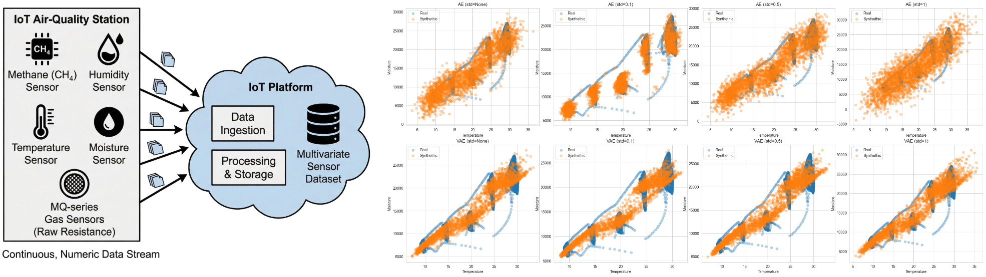
In this post we will see that Generative Adversarial Networks (GAN) have serious problems with mode collapse, which affects the diversity of synthetic data. While Denoising Diffusion Model (DDM) can cover a wide spectrum of possibilities, they suffer from thousands of network evaluations respectively. On the last term, Variational Auto-Encoders (VAE) and likelihood-based models are fast samplers but are limited when creating diverse patterns not present in the training data.

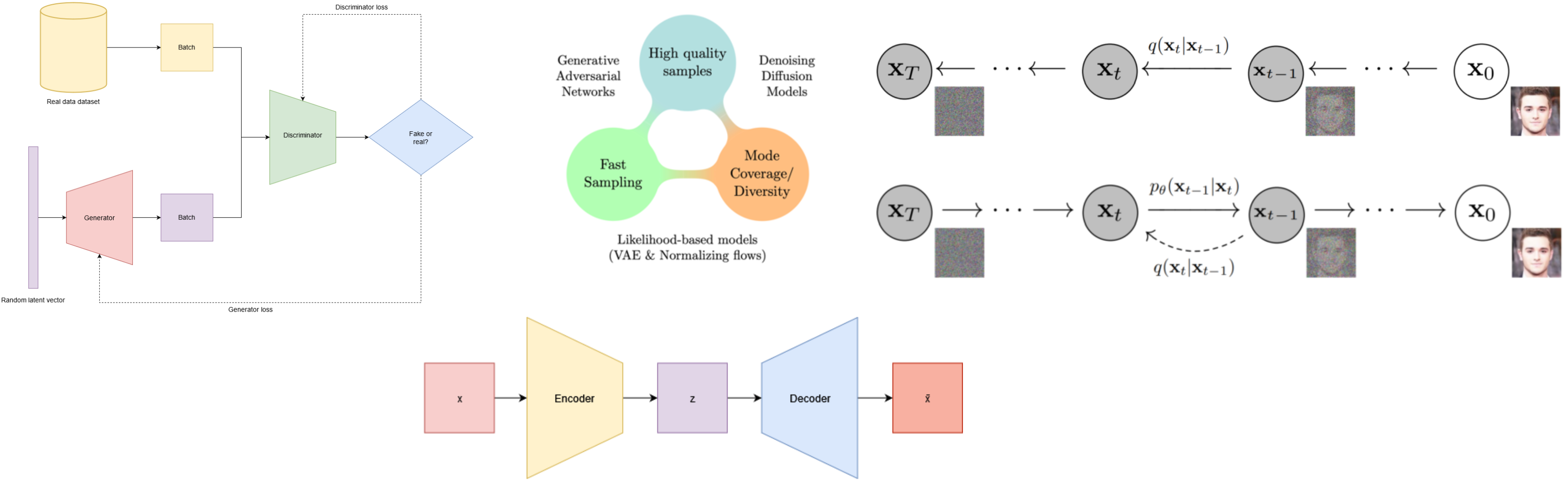
Most of the current deep generative learning models focus on high-quality definition, although all the requirements are highly important and key factors in a real environment. All of them have their advantages and drawbacks - and this is called the generative learning trilemma.

Warning! This post is a re-written part from my master’s thesis that you can also find here.

Generative Adversarial Network

A GAN is an unsupervised model made up of two neural networks: the generator and the discriminator. The idea is based on a game theoretic scenario in which the generator network must compete against an adversary. While the generator network produces samples, the aim of the discriminator is to distinguish between the real samples and the drawn by the generator. The discriminator is a binary classifier trying not to be fooled.

The generator loss is calculated using the discriminator as a reference of how much far is from real images while the discriminator loss is calculated by how much accurate is discerning between the synthesized data and the real one. The standard function can be known as the min-max loss:

\[Loss_D(D) = E_x[log(D(x)]\]

\[Loss_G(G) = E_y[log(1 - D(G(y)))]\]

\[Loss_{GAN}(G, D) = Loss_D(D) + Loss_G(G)\]

During training, both networks constantly try to outsmart each other, in a zero-sum game. At some point of the training, the game may end up in a state that game theorists call a Nash equilibrium, when no player would be better off changing their own strategy, assuming the other players do not change theirs. GANs can only reach one possible Nash equilibrium: when the generator produces so realistic images that the discriminator is forced to guess by 50 % probability that the image is real or not.

Nevertheless, the training process not always can converge to that equilibrium. There are several factors that make the training hard to reach the desired state. For instance, there is a possibility that the discriminator always outsmarts the generator so that it can clearly distinguish between fake and real images. As it never fails, the generator is stuck trying to produce better images as it cannot learn from the errors of the discriminator.

Possible solutions can be carried out such as making the discriminator less powerful, decreasing the learning rate or adding noise to the discriminator target. Another big obstacle is when the generator becomes less diverse, and it learns only to perfectly generate realistic images of a single class, so it forgets about the others. This is called mode collapse.

At some point, the discriminator can learn how to beat the generator, but then, the latter is forced to do the same but in another class, cycling between classes never becoming good at any of them. A popular technique to avoid is experience replay, which consists in storing synthetic images at each iteration in a replay buffer.

There is a lot of literature of obstacles and solutions to improve GAN training and it is still very active, as it is in its applications too. The tuning of hyper-parameters and the design of the model will be a key to pursue the Nash equilibrium.

For instance, there is a variant called cGAN (conditional GAN). Traditionally, the generative network only produces the image from a random vector as an input, which is also called latent vector since it cannot be manipulated or with prior convictions of how will be. Unfortunately, this only allows to generate a random image from the domain of the latent space, which is hard to map to the generated images. However, cGAN can be trained so that both generator and discriminator models can be conditioned to some class labels or multi-dimensional vectors and produce synthetic images from a specific domain. In the following figure, it can be seen a cGAN diagram where the generator is conditioned by some inputs as well as the real data have the condition vector in each sample.

Variational Auto-Encoders

Likelihood-based models are alternatives to GANs that can cover a wide range of possibilities since they focus on estimating the likelihood or probability distribution of the data while training. There are several types of likelihood-based models although we will focus on VAE. The architecture of autoencoders are quite simple, they consist of an encoder, a smaller feature vector also called latent vector \(z\) and a decoder , as it can be seen in Figure 5. Therefore, the main goal of the encoder is to comprise the input vector \(x\) while the decoder attempts to perform the conversion from lower to higher dimensional data, being the output vector \(\bar{x}\). Hence, the best purpose of autoencoders is dimensionality reduction given its architecture. Then, the main purpose is to find the best set of encoder/decoder that keeps the maximum information with the less reconstruction error while decoding. In fact, one of the most popular usages of autoencoders in computer vision is the image reconstruction due to their architecture.

Let’s assume an autoencoder that both encoder and decoder have only one layer without non-linearity. In that sense, we can see clearly a link with PCA since we are looking for the best linear subspace to project data on with as few information loss as possible.

However, deep neural networks comes with also non-linear layers (non-linear layers allow to learn complex relationships. Some of them are used as activation functions). The more complex of autoencoders architecture, the more they can proceed to a high dimensionality reduction while keeping the loss low. In an ideal case, if the encoder and the decoder have enough degrees of freedom and infinite power, the latent vector could be reduced to one. Nevertheless, the dimensionality reduction comes with a price.

First, we will lack of interpretable structures in the latent space. Secondly, the major part of the data structure information will not be in a reduced representation but in arbitrary one without any context of the patterns that the autoencoder could infer. Therefore, it is important to control and adjust the depth and the latent space dimensions depending on the final purpose.

At this point, we have learned the surface from autoencoders, but how do they fit in image generation? Once the autoencoder has been trained, we have both encoder and decoder with the weights to reconstruct the data. At first, we might think that changing the latent vector we could take a point randomly from the space and decode it to get a new content. Although that could work, the regularity of the latent space for autoencoders is hard since it depends on several factors such as the data distribution, the latent space dimension and the architecture of the encoder. To sum up, there will be several biases that we are not able to control.

In order to make the latent vector regular and continuous, VAEs try to solve this problem by mapping the inputs to a normal probability distribution, so they introduce explicit regularization during the training process. Hence, the latent vector will be sampled from that distribution, being the decoder more robust at decoding latent vectors as a result. A VAE is an architecture composed of both encoder and decoder too. However, instead of encoding a latent vector, they encode it as a distribution over the latent space. The following enumeration details the process:

1. The input is encoded as a distribution over the latent space.
2. A point is generated given the distribution encoded.
3. The sampled point is decoded so the reconstruction and regularization error can be computed.

The encoded distributions are chosen to be normal so that the encoder can be trained to return the mean and covariance matrix. This makes a way of both local and global regularization of the latent space respectively. Hence,the loss will not be only about the reconstruction of the data in the last layer, called reconstruction term, but also how the latent space is organized by making the latent space close to a standard normal distribution, called the regularization term. The latter will be calculated by how distant is from the gaussian distribution. Kullback-Leibler Divergence, is a measure of how one probability distribution differs from a second, reference probability distribution. It’s commonly used in various fields, including information theory, statistics, and machine learning. Using the KL divergence, which is expressed in terms of the means and the covariance matrices of the two distributions, the variety of outputs are better represented in the latent space in VAEs than traditional autoencoders:

\[L_{\text{VAE}} = \text{Reconstruction term} +\qquad \text{Regularization term}\]

\[\text{Reconstruction term} = (\frac{1}{N} \sum_{i=1}^{N} \| x_i - \bar{x}_i \|^2)\]

\[ \text{Regularization term} = \sum_{j=1}^{J} \left(\mu_j^2 + \sigma_j^2 - \log(\sigma_j) - 1 \right)\]

The loss in VAEs is also called the variational lower bound or ELBO as a way to estimate the likelihood of the observed data given the model’s parameters and latent variables. To demonstrate the differences we can compare an autoencoder and a VAE trained by MNIST data, although it is a really balanced dataset. We can see in that the range of values in the latent vector of the latter is much smaller and centralized, representing better any class, whereas autoencoder has the images more sparsed in the latent domain.

Moreover, one particularity that makes VAE architectures good in business and industry related problems or even in processing images (one problem that VAE solve really well is in image reconstruction since it gets the main and reduced idea of an image) is that they are really fast when sampling due to its bottleneck and the dimensional reduction feature. Nevertheless, the reduction of the bottleneck also makes that the quality of the samples produced by VAE are lower than other generative models. In particular, when they are compared to DDMs.

Denoising Diffusion Models

Denoising Diffusion Models (DDMs) are a type of generative model that operates through a different framework than VAEs, although their basis is also probabilistic. While VAEs focus on encoding data into a latent space and then decoding it to generate reconstructions, DDMs revolves around modeling the diffusion process of data. This process involves the gradual transition from a noisy version of the data to the actual clean data. The process of training a DDM involves optimizing the parameters of the diffusion process so that it can effectively recreate the observed data distribution. But, what is this process about? We can assume that all data comes from a distribution. Basically, any dataset is sampled from the real distribution. The goal of generative models is to learn that distribution so they could sample from it and get another data point that looks like is from the dataset trained. The way that DDM learns that distribution is by trying to convert well-known and simple base distribution (like gaussian) to the target data iteratively, with small steps, using a Markov chain, treating the output of the markov chain as the model’s approximation for the learned distribution. Hence, the diffusion process can be split into two parts: forward and reverse diffusion processes.

In the forward process \(q(x_{t}|x_{t-1})\), the model slowly and iteratively add noise to the images so that they move out from their existing subspace.

Since it is proved that doing it infinitely the image would eventually end up into a point from a normal distribution \(q(x_T|x_0) \thickapprox \mathcal{N}(0,1)\), the final corrupted image would loss all information from original sample. So, what it is aimed is to convert the unknown and complex distribution of the dataset into one that it is easier to sample a point from and understand. The forward process takes the form of a markov chain, where the distribution at a particular time step only depends on the sample of the immediately previous step. Therefore, it is easy to write out the distribution of corrupted samples conditioned on the initial data point \(x_0\) as the product of successive single step conditionals:

\[q(x_{1:T} | x_0) = \prod_{t=1}^{T} q(x_t|x_{t-1})\]

In the case of continuous data, each transition is parameterized as a diagonal gaussian probability distribution function and that is the reason why approximating to \(T\) would end up to a gaussian distribution centered at 0, since the parameter \(\beta\) will always approach to \(1\) and, then, \(\sqrt{1 - \beta_T}\) theoretically will approach to 0:

\[q(x_{t}|x_{t-1}) = \mathcal{N}(x_t; \sqrt{1 - \beta_t} x_{t-1}, \beta_t I)\]

\[ \beta_1 < \beta_2 < ... < \beta_T \quad ; \quad \beta_t \in (0,1) \]

Although taking small steps has a cost, learning to undo the steps of the forward process would be less difficult. Adding little noise at each step, there would be less ambiguity about determining the probability density function of the last step in the reverse process.

The goal of the reverse process is to undo the forward and to learn the denoising process in order to generate new data from random noise. Unfortunately, infinite paths can be taken starting from the corrupted image but only few of them will turn the noisy image into a data from the desired subspace. Hence, DDM takes small iterative steps during the forward diffusion processes and take those steps which the probability distribution function satisfies that the corrupted images differs slightly at each step.

Like the forward process, the reverse process is set up as a markov chain, being the pure noise distribution \(p(x_T) = \mathcal{N}(x_T; 0, 1)\):

\[p_{\theta}(x_{0:T}) = p(x_T) \prod_{t=1}^{T} p_{\theta}(x_{t-1}| x_t)\]

\cite{feller1950} shows that theoratically the true reverse process will have the same functional form as the forward process. Therefore, the each learned reverse step will be also a diagonal gaussian distribution:

\[p_{\theta}(x_{t-1}|x_t) = \mathcal{N}(x_{t-1}; \mu_{\theta}(x_t; t), \sigma_{\theta}(x_t, t))\]

The forward objective is to push a sample off the data manifold turning into noise and the reverse process is trained to produce a trajectory back to the data manifold, resulting in a reasonable sample. The objective that we attempt to optimize is not about optimizing the maximum likelihood objective to turn a point to \(x_0\), because \(p_{\theta}(x_0) = \int p_{\theta}(x_{0:T}) dx_{1:T})\) includes all the possible trajectories, all the ways a noisy point could have arrived at \(x_0\). If we compare VAE with DDM, the encoding part would be the forward process while the decoder would be the reverse model. Hence, the latent variables would be \(\{x_i | i \in \{1, 2, ..., T\}\}\) while the observed variable, \(x_0\). Unlike a VAE, the encoder part is typically fixed but the reversed process is the one being focused while training, so a single network needs to be trained. When we have a model with observations and latent variable, we can use the ELBO to maximize the expected density assigned to the data while the KL divergence encourages the approximate posterior \(q(z|x)\) to be similar to the prior on the latent variable \(p_{\theta}(z)\).

Therefore, any step forward and back would include a loss of the divergence between both distributions. Nevertheless, although at training time any term of this objective can be obtained without having to simulate an entire chain, different trajectories may visit different samples at time \(t-1\) on the way to hitting \(x_t\), the setup can have high variance. limiting training efficiency. To help with this, the objective must be arranged as follows.

\[E_q[-D_{KL}(q(x_{T}|x_0) \; || \; p(x_T)) - \sum_{t > 1} D_{KL}(q(x_{t-1} | x_t, x_0) \; || \; p_{\theta}(x_{t-1} | x_t)) + log \, p_{\theta}(x_0| x_1)]\]

The first part it compares the noise distribution (The start of the reverse process) \(p(x_T)\) with the forward process \(q(x_T|x_0)\), which both are fixed. The second component is a sum of divergences each between a reverse step and a forward process posterior conditioned on \(x_0\). When the \(x_0\) is treated as known like it is during training, all \(q\) terms are actually gaussians. Then, the divergences is comparing two gaussians and helps reducing variance during the training process.

In order to add conditional inputs in the model is to feed the conditioning variable \(y\) as an additional input during training \(p_{theta}(x_0 | y)\). Moreover, adding a separate trained classifier can help guiding the diffusion process in the direction of the gradient of the target label probability with respect of the current noise image.

Comparing DDMs and VAEs, DDMs can capture complex dependencies and distributions in the data due to their inherent modeling of the diffusion process. Estimating and analyzing small step sizes is more tractable than describing a single non-normalizable step from random noise to the learned distributions, which is what VAEs and GANs do. However, they can be computationally more intensive to train due to the intricacies involved in estimating the diffusion process parameters accurately.

Conclusion

The exploration of Generative Adversarial Networks (GANs), Variational Auto-Encoders (VAEs), and Denoising Diffusion Models (DDMs) illustrates the inherent trade-offs within the Generative Learning Trilemma: the balance between sample quality, sampling speed, and mode coverage/diversity.

Each model type occupies a distinct position within this trilemma:

• GANs excel at generating visually realistic, high-quality samples but struggle with mode collapse, often failing to represent the full diversity of the data. Their adversarial training is also notoriously unstable, requiring careful balancing between generator and discriminator dynamics.
• VAEs prioritize efficient sampling and structured latent spaces, offering fast generation and interpretability. However, their reconstructions tend to be overly smooth or blurry, reflecting the limitations of their probabilistic assumptions and the imposed regularization on the latent space.
• DDMs, in contrast, achieve exceptional diversity and fidelity by explicitly modeling the data generation process as a gradual denoising sequence. Their main drawback lies in computational cost, as thousands of iterative steps are needed for both training and sampling.

In essence, these three paradigms represent different compromises among realism, efficiency, and coverage.

The future of generative modeling likely resides in hybrid architectures that integrate the strengths of each approach. As computational power and architectural innovations continue to evolve, these generative models will converge toward systems capable of high-quality, diverse, and efficient generation, moving closer to resolving the generative trilemma that defines this fascinating field.