Embedding models are foundational in modern NLP, turning raw text into numerical vectors that preserve semantic significance. These representations power everything from semantic search to Retrieval-Augmented Generation or Prompt Engineering for LLM Agents. With growing demand for domain-specific applications, understanding which is the best fit for your system is more important than ever.

Introduction

In modern NLP, a text embedding is a vector that represents a piece of text in a mathematical space. The magic of embeddings is that they encode semantic meaning: texts with similar meaning end up with vectors that are close together. For example, an embedding model might place “How to change a tier” near “Steps to fix a flat tire” in its vector space, even though the wording is different. This property makes embedding models incredibly useful for tasks like search, clustering or recommendation, where we care about semantic similarity rather than exact keyword matches. By converting text into vectors, embedding models allow computers to measure meaning and relevance via distances in vector space.

However, not all embeddings are created equally, and using a generic embedding model for every task can be limiting. Many pre-trained embedding models are trained on broad internet text or general knowledge. If you application works in a specific domain (finance, medical, legal, etc.) those models might not capture the nuances or terminology that matter for your context. This is where fine-tuning comes in. By fine-tuning an embedding model on data from your domain, you can make it specialist rather than generalist, aligning the vector space with what’s actually important for your documents and queries.

This post explores the landscape of embedding models, from their historical evolution (Word2Vec, GloVe) to modern transformer-based architectures (BERT, SBERT, E5, ColBERT). You’ll learn how they differ, how to choose between them and improve your RAG-based system.

The importance of vectors that understand

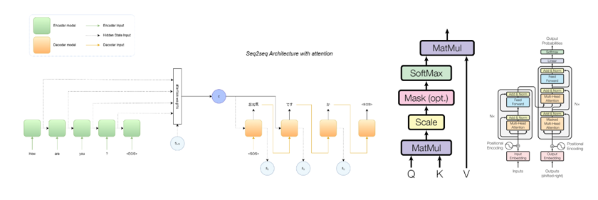
At a high level, an embedding model is a neural network that encodes text into a high-dimensional vector. The goal is to represent text in a numerical form that captures linguistic and semantic characteristics. Early examples include word2vec and GloVe, which learn static word embeddings (each word type in the vocabulary gets a fixed vector representation). Modern examples include transformers like BERT, RoBERTa or Sentence-BERT, which can produce embeddings for entire sentences or paragraphs and its output depends on the attention mechanism applied between tokens.

Similarity between texts can be measured by vector distances metrics such as cosine similarity or euclidean distance. In an embedding space, similar texts are designed to lie close together, while dissimilar texts are far apart. This enables semantic search: se can take a user query, embed it into a vector, and quickly find which documents have embeddings nearest to that’s query embedding. This approach goes beyond keyword matching; it can retrieve information that uses different wording but conveys the same idea.

Embeddings also shine in other tasks like clustering (grouping similar documents), classification (feeding embeddings into machine learning models) or anomaly detection. They condense the essential information of text into a numeric form that algorithms can easily work with. Additionally, embedding models are not just for text but for image (for example, vehicle re-identification), so the number of usages is exponentially greater than it is thought to be. Overall, embedding models are key to understanding text or image in ML systems, offering a vector-based representation that preserves meaning.

Taxonomy of Text Embeddings

Not all embedding models work the same way. We can categorize them along a few dimensions: how they treat context (static vs. contextual embeddings), what textual unit they embed (word-level vs. sentence-level), how are they trained ( unsupervised or supervised), the nature of the vector representations (dense vs. sparse embeddings), the interaction during scoring (single vector comparison vs. token-level max similarity, also called late interaction) and their type of purpose (symmetric vs. asymmetric). Understanding this taxonomy will clarify the landscape of embedding techniques and when to use each.

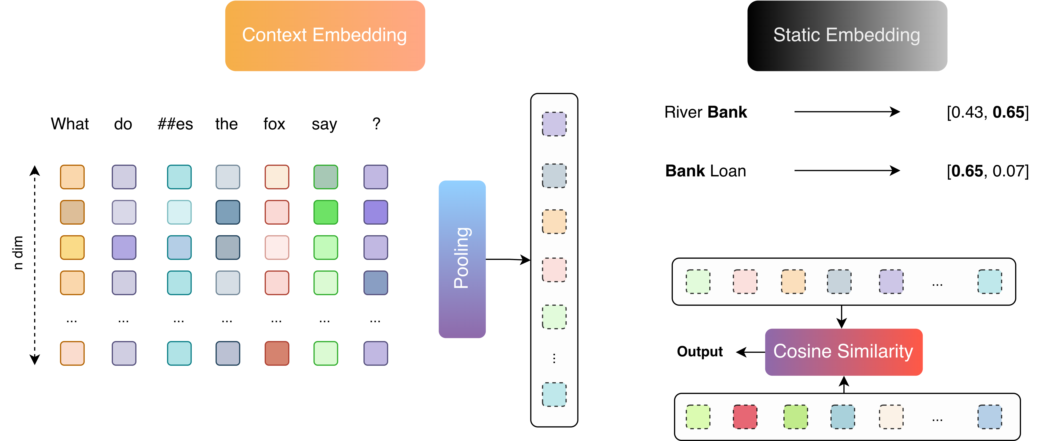
Static vs Contextual word embeddings

Static embeddings were the early wave of embedding models exemplified by Word2Vec, GloVe, and FastText. These models learn one vector per word in a fixed vocabulary by training on large corpora to capture general semantic relationships. The key characteristic is that each word has a single embedding no matter where it appears. The word “point” will have the same vector representation whether we’re talking about a “point of reference” or a “point on a graph”. Static embeddings thus ignore context: they can’t distinguish between different meanings of the same word in different sentences.

Contextual embeddings, on the other hand, produce vectors that depend on the surrounding context of each word. Transformer-based models output a contextualized embedding for each token (and often for entire sentences) by considering the whole sentence or paragraph. In a contextual model, the word “point” will have a different embedding in “make a point” vs. “point guard” vs. “point of intersection,” because the model understands these are different usages based on context. This is achieved through mechanisms like self-attention that let every token influence the representation of others. Contextual embeddings were a major breakthrough because they capture nuances and resolve ambiguity that static embeddings cannot.

In practice, contextual models (like BERT) yield much stronger performance on language understanding tasks than static embeddings, since meaning often depends on context. The trade-off is that they are heavier to compute; generating contextual embeddings requires running a full transformer over the text, whereas static embeddings can be looked up from a table. Nonetheless, for most NLP applications today contextual embeddings are the default choice due to their accuracy and expressiveness. Static embeddings are still useful for quick, lightweight needs or as features in simpler models, but they lack the fidelity that modern tasks demand.

Word-Level vs Sentence-Level embeddings

Another way to classify embeddings is by the unit of text they represent. Traditional word embeddings (static or contextual) give you a vector for each word (or token) in a sequence. But we often need a single embedding for a whole sentence, paragraph, or document: for example, to compare a user’s query with a candidate answer passage, it’s handy to represent each passage as one vector.

How do we get a vector for an entire sentence or document? One approach is to take a contextual model like BERT and pool its token embeddings into a single vector (e.g. use the [CLS] token output or average the token vectors). However, out-of-the-box BERT wasn’t trained to produce a single “sentence meaning” vector, and in fact a naive use of BERT’s [CLS] embedding can give subpar results for similarity tasks. Recognizing this, researchers developed models and training techniques specifically for sentence embeddings. A notable example is Sentence-BERT (SBERT), which fine-tunes BERT (or similar architectures) on sentence pair tasks so that it directly produces a meaningful sentence-level embedding. SBERT uses a siamese network setup and a contrastive loss so that similar sentences map to nearby vectors. The result is a model that can encode an entire sentence or paragraph into a single vector that is excellent for semantic similarity comparisons, clustering, etc.

So, we distinguish word-level vs. sentence-level embedding models. Word-level models (like the original BERT, although currently serves as a Sentence-level model) give flexibility: you can derive embeddings for any granularity (subword, word, sentence) but might need task-specific tuning to get good sentence representations. Sentence-level models are explicitly optimized to output one vector for a whole input text that captures its meaning. In RAG pipelines for QA, we typically need to compare questions and passages. Using a sentence-level embedding model (or more generally, a model that produces one vector per query or document) is thus a natural choice. Indeed, Sentence-BERT and similar models are popular for dense retrievers because they strike a balance: they leverage deep context understanding from transformers but output compact vectors for entire texts, making them directly usable in a retrieval setting.

Unsupervised (self-supervised) Pre-Training vs Supervised Contrastive Learning

Beyond architecture, embedding models are distinguished by how they are trained: the learning objective and data used greatly influence the resulting vector representations.

Many embedding models are first trained without any human-labeled data, using self-generated signals from raw text (or other modalities) to learn representations. A common self-supervised objective is language modeling. For instance, BERT was trained with Masked Language Modeling (MLM) (randomly masking words in a sentence and training the model to predict them, thereby forcing it to absorb contextual semantics) and a secondary next-sentence prediction task. This kind of unsupervised training on large corpora (Wikipedia, Books, web text, etc.) yields a general-purpose language understanding capability. However, the resulting embeddings are not explicitly tuned for similarity or retrieval out-of-the-box. Indeed, a vanilla BERT’s sentence embeddings needed further fine-tuning to be effective for semantic similarity. Unsupervised training uses massive unlabeled corpora. For BERT, this was billions of words of BooksCorpus and Wikipedia. For unsupervised SimCSE, it was a large generic text corpus (natural sentences). These models are often evaluated intrinsically by language modeling perplexity or downstream transfer performance.

Supervised training for embeddings leverages labeled pairs or tuples of texts that indicate which items should be similar or dissimilar in the vector space. A prevalent approach is contrastive learning with positive and negative pairs: the model is trained to produce embeddings that are close (in cosine or dot-product space) for semantically related pairs, and far apart for unrelated pairs. This can be implemented via a contrastive loss or as a softmax cross-entropy over a batch where each input should be closest to its true match among the batch negatives. For example, Sentence-BERT (SBERT) was fine-tuned on Natural Language Inference (NLI) data where sentence pairs have labels Entailment/Neutral/Contradiction. It took sentence pairs as input to a Siamese network and trained with a classification loss that implicitly makes entailment pairs come closer in embedding space and contradiction pairs repel. Another example is Dense Passage Retrieval (DPR) for question answering: DPR used question–answer pairs from Wikipedia; it trained dual BERT encoders for question and document, with a loss that pushes the question embedding near its correct passage’s embedding and away from other passages.

Dense vs Sparse embeddings

A third key distinction is dense versus sparse embeddings. This refers to the nature of the vector itself.

Dense embeddings are the kind we’ve been mostly discussing (continuous vectors in a dimensional space). Every value in the vector is typically a non-zero real number (after training), and the information is distributed across the dimensions. Neural network models naturally produce dense vectors. For example, a BERT-based sentence embedding might be a 768-dimensional dense vector with values like [0.5, -0.8764, ..., 0.065]. Dense vectors excel at capturing semantic similarity through all those learned dimensions; two pieces of text about the same topic will have correspondingly similar coordinates along those axes.

Sparse embeddings are high-dimensional vectors where most entries are zero. Traditional bag-of-words representations, like TF-IDF vectors, are classic sparse representations: you might have a 100,000-dimensional vector where each dimension corresponds to a vocabulary term, and you set a value (e.g. a TF-IDF weight) in those dimensions where the term is present in the document. These vectors are sparse because any given document uses only a few words out of the whole vocabulary, so it might have non-zero values in, say, 100 out of 100,000 dimensions (the rest being zero). Sparse embeddings thus align closely with lexical representations: they emphasize exact term matching and frequency.

In the context of retrieval, dense and sparse methods have different strengths. Dense embeddings (a.k.a. “semantic embeddings”) capture meaning, even if wording differs. They can retrieve relevant texts that don’t share any exact keywords with the query, by focusing on semantic closeness. Sparse methods (lexical retrieval like BM25) excel at precision for the exact query terms (if a query contains a rare term, a sparse method will almost certainly find docuemnts containing that term). But sparse methods won’t generalize to synonyms or rephrasings (if you search for “vehicle tire”, a pure BM25 search might miss a document that only says “automobile wheel”). Dense methods might catch that thanks to semantic training, but dense methods can sometimes retrieve things that are topically related yet not exact, which could be irrelevant if not carefully filtered.

Modern best practice often uses a hybrid approach: combine dense and sparse retrieval to get the best of both worlds. For example, you can rank documents by a weighted sum of semantic similarity (dense vector dot product) and lexical similarity (BM25 score). This can improve accuracy because some queries are best served by semantic matching, and some by precise keyword matches. There are also neural models like SPLADE that try to bridge the gap by producing sparse vectors in a learned way. Essentially, SPLADE tries to predict which vocabulary terms should be given weight for a document, combining the idea of expansion terms with a neural model. Other approaches like BM42, use IDF and attention from dense embedding models to calculate their similarity score, trying to improve the query inference speed from SPLADE and large documents accuracy. However, many teams stick to joining both techniques separately and then using a re-ranker to join both results. In summary, dense embeddings vs. sparse embeddings is not a competition with a single winner; they are complementary tools. Knowing their differences helps in choosing an appropriate retrieval strategy for your application.

Single vector comparison vs Late Interaction models

Late interaction computes relevance by comparing fine-grained token-level embeddings, rather than comparing two global sentence/document embeddings. Sentence-level models (e.g., SBERT, E5) are designed for global semantic similarity, not fine-grained token alignment. Late interaction models, on the other hand, like ColBERT retain token-level embeddings and compute relevance scores by aggregating interactions between individual tokens of the query and document.

Late interaction defeats the purpose of sentence-level embeddings, which aim to summarize a whole text span into a single dense vector for fast retrieval (e.g., via approximate nearest neighbor). ColBERT doesn’t pool token embeddings into a single vector, it keeps all token-level BERT embeddings and then, during retrieval computes fine-grained similarity between every query token and all document tokens, also called maximum cosine similarity. Late interaction is slower and more computationally expensive due to per-token comparison. This cost makes little sense for short texts like single sentences.

Overall, what is important to understand is that the key difference between BERT and late interaction embedding models lies in how they use BERT’s outputs, not in the architecture itself. Some hybrid approaches may use sentence-level embeddings for fast coarse filtering, then perform token-level re-ranking (but that’s post-retrieval, not part of the embedding model). It is especially useful in RAG where precise grounding improves generation.

In this this post from Qdrant, you can see how you can turn single-vector dense embedding models into late interaction models.

Symmetric vs. Asymmetric embedding models

Symmetric vs. asymmetric embedding models represent two different approaches for encoding queries and documents. In symmetric embedding architectures, both inputs (e.g. a query and a document) are processed using the same model or encoder pipeline. In other words, the query and document are handled identically. For example, Sentence-BERT (SBERT) encodes two sentences using the same Transformer network and produces embeddings that can be directly compared. This works well when the inputs are homogeneous. Therefore, symmetric models are natural for tasks like finding duplicate questions, matching similar product description or clustering semanticallu similar texts.

By contrast, asymmetric embedding architectures use different encoders or processing for the query vs. the document. This design is typical when the inputs differ in format, length, or role. The motivation for asymmetric models arises when queries and documents have inherently different distributions or functions. A user’s query is usually short, may omit context, and represents an information need or intent, whereas a document passage is longer, detailed, and represents content that might satisfy that need. Here an asymmetric model might use a lightweight query encoder and a heavier document encoder optimized for content, projecting both into a shared vector space. The key idea is role specialization: each encoder can focus on encoding its input (query or doc) in the most effective way, rather than one model trying to serve both roles.

Concretely, using a symmetric embedding for a QA task can lead to suboptimal results. Such models tend to emphasize semantic similarity between query and document text, rather than relevance of a document as an answer. For example, a symmetric model trained for general sentence similarity might, given the query “What is Python?”, rank another question like “What is Python used for?” highly, because those two questions are lexically and semantically similar. An experiment comparing models illustrates this: a paraphrase-trained (symmetric) MiniLM model was tested vs. an MS MARCO-trained (asymmetric) MiniLM model on the query “What is Python?”” The symmetric model ranked similar questions highest, whereas the MS MARCO model (fine-tuned on question–answer pairs) gave a much higher score to the actual answer passage.

The reason is that asymmetric training can decouple “intent” vs. “content.” An asymmetric embedder can learn a specialized query representation that encodes the information need (e.g. focusing on the key question terms), and a document representation that encodes content (the factual answer, even if paraphrased). The two embeddings might not be extremely similar in raw semantics (a question and its answer have different wording and meaning), but the model learns to make them compatible in the shared vector space.

Another motivation is distributional differences like length and vocabulary. Queries are often just a few words, documents have many. A single encoder might have trouble handling both extremes. An asymmetric approach can use a specialized query encoder (perhaps one that is simpler and emphasizes keywords) and a separate doc encoder (that fully encodes the description). In general, allowing asymmetry lets each side play to its strengths: the query encoder can be optimized for short, context-poor inputs, and the document encoder for long, rich text.

Asymmetric models intentionally introduce differences in the encoders or encoding process between the query side and the document side. The simplest form of this is to have two different neural encoders – one dedicated to queries and another to documents. Each may have its own parameters, or even a different architecture, though they are usually coordinated to output comparable vectors (often of the same dimension) for similarity scoring. The output embeddings reside in a shared vector space, but how they are produced can differ.

A clear example is E5 (Embeddings from bidirectional Encoder representations, 5 stands for five E’s in the acronym). On the surface, E5 uses a single Transformer encoder for both query and passage text, which sounds symmetric. However, it introduces an ingenious asymmetry: a special token prefix on each input to indicate its type (e.g. prepend "query: " to questions and "passage: " to passages). Thus, although the weights are shared, the model learns to handle the two roles differently based on the prefix cue. During pretraining on a huge weakly-supervised dataset, E5 sees query–passage pairs (like search query and relevant result, or question and its answer) and uses a contrastive dual-encoder objective to bring the query embedding close to its paired passage embedding.

The use of role-specific prefixes is not strictly required, but “often helps in IR settings”, and users are advised to include them for best performance. n effect, E5 behaves as an asymmetric model: if you encode some text as a “query,” the embedding lives in the same vector space but on a slightly different manifold than if you encode it as a “passage.” This helps the model capture that, for example, the word “Python” in a query might mean the user is asking about Python (intent), whereas “Python” in a passage likely indicates the content (definition or usage of Python).

A case in point is DPR (already talked in Supervised Contrastive Learning), a popular model for open-domain QA. DPR consists of two BERT-base encoders (one for questions and one for passages) which are initialized with the same architecture but are independently learned (no weight sharing). DPR consists of two BERT-base encoders (one for questions and one for passages) which are initialized with the same architecture but are independently learned (no weight sharing). Some people consider these models as symmetric even if they don’t share weights, since DPR still projects questions and passages into a single common vector space, enabling similarity search. This means it can be seen as an un-tied symmetric model (the encoding function form is the same for queries and docs, though optimized separately). However, what DPR models try to solve is the same as asymmetrical embedding models: match the intent with the content. So, it seems more like a philosophical consideration rather than a pragmatical point of view.

In summary, asymmetric architectures can be implemented by: (1) distinct encoder networks for each side, (2) augmenting a shared encoder with input-specific signals or just (3) train or fine-tune the model with query - passage dataset without considering paraphrased pairs.

Key Takeaways and Future Directions

Embedding models have transformed how machines represent and reason about meaning. From early static vectors like Word2Vec to modern transformer-based systems like Sentence-BERT and E5, embeddings now serve as the semantic interface between human language and machine reasoning.

Understanding their taxonomy (static vs. contextual, word-level vs. sentence-level, dense vs. sparse, symmetric vs. asymmetric) is crucial for choosing the right model for your task. While dense embeddings capture deep semantics, sparse ones preserve interpretability and precision. Similarly, symmetric models work best for homogeneous text comparisons, while asymmetric architectures excel in information retrieval and RAG.

In practice, the future of embeddings lies in hybrid systems: combining dense and sparse methods, using domain-adapted fine-tuning, and integrating late-interaction models for fine-grained relevance. These advances are not just technical upgrades: they reshape how AI systems understand, search, and generate knowledge.

Whether you are building a semantic search engine, a retrieval-enhanced chatbot, or a domain-specific RAG pipeline, mastering embedding models means mastering the core bridge between text and meaning.

@article{alas2025,
  title   = "From Words to Vectors: A Dive into Embedding Model Taxonomy.",
  author  = "Alàs Cercós, Oriol",
  journal = "oriolac.github.io",
  year    = "2025",
  month   = "October",
  url     = "https://oriolac.github.io/posts/20251025-embedding-models/"
}