The post of today is going to be a bit different. We have already talked about Variational Autoencoders (VAE) in the past, but today we are going to see how to implement it from scratch, train it on a dataset and see how it behaves with tabular data. Yes, VAEs can be used for tabular data as well. To do so, we will use the CRISP-DM framework to guide us through the process.
Business Understanding
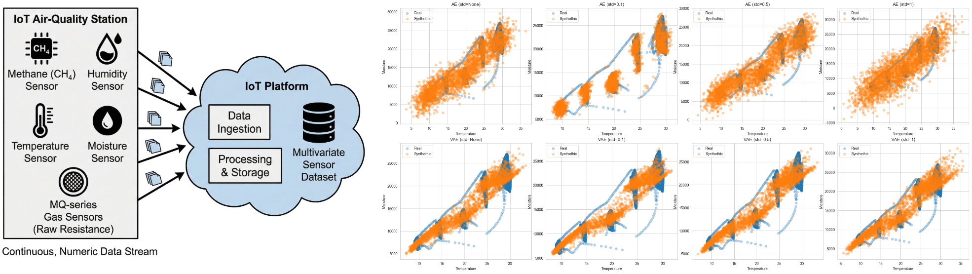
The dataset used in this project is obtained from a public GitHub repository and contains multivariate measurements collected by a low-cost IoT air-quality station. These stations typically combine semiconductor gas sensors (e.g., MQ-series) with environmental sensors to capture methane concentration, humidity, temperature, and moisture, along with raw sensor resistance readings.

Methane (CH₄) is a key atmospheric gas with strong implications for environmental monitoring, industrial safety, and public health. Sudden increases in methane concentration can indicate gas leaks, malfunctioning equipment, incomplete combustion, or abnormal environmental conditions.
Methane is influenced by several environmental and sensor-derived variables, and therefore offers a realistic dependency structure. However, the goal of this project is not to build a production-ready predictive model, but rather to create a controlled scenario that allows us to understand how Variational AutoEncoders (VAE) behave when trained on multivariate IoT sensor data and how other regression models can improve their performance using synthetic data. To do this we will generate synthetic datasets that mimic real sensor readings and then define a lightweight regression task focused on methane concentration.
Data Understanding
The dataset consists of eight environmental and sensor-derived variables together with a target variable representing methan concentration (in ppb). All variables are continuous and numeric but the dataset does not include timestamps. Therefore, we will assume (for this post) that the data is not a time-series dataset and the model cannot leverage temporal patterns, lagged dependencies, or sequence-based correlations. Maybe in future posts I will use this data considering the consecutive rows as next timestamps.
import pandas as pd

df = pd.read_csv(
    "https://raw.githubusercontent.com/gungunpandey/Synthetic-Data-Generation/refs/heads/main/Dataset%201.csv")
Correlation matrix
If we create the correlation matrix between all the variables, the first thing we see is how the two variable families are also split by their correlations between them:
- Environmental and context variables: Moisture, temperature and humidity
- Gas-sensor electrical signals: R2611E, R2600, R2602, R2611C, RMQ4
- Target variable: Methane (ppb)
import matplotlib.pyplot as plt
import seaborn as sns

plt.figure(figsize=(10, 8))

corr = df.corr()

sns.heatmap(
    corr,
    annot=True,
    fmt=".2f",
    cmap="coolwarm",
    vmin=-1, vmax=1,
    square=True,
    linewidths=0.5,
    cbar_kws={"shrink": 0.8}
)

plt.title("Correlation Heatmap", fontsize=16)
plt.tight_layout()
plt.show()
The matrix shows strong structure: the resistance channels move together, and they move opposite to temperature/moisture. While temperature and moisture have strong positive correlation between them and strong negative correlation with gas-sensor electrical signals, humidity does not have such strong relationship with the variables.
Although it seems a difficulty added to the data, it can be helpful since we are adding a new layer of complexity to understand how methane can behave. If humidity does not exist, might be better to use a PCA rather than VAE!

My interpretation of most of the resistance channels is that they are responding to a common driver (often a mix of gas exposure + environment). R2611C and RMQ4 are near-duplicates; R2602 may be the only one adding a meaningfully different dimension.
Regarding our target variable, we can see that methane has moderate negative correlation with several resistance channels and almost independent from humidity and really weakly to moisture and temperature.
Variable distributions
I have used KDE plots to show the data distribution on each of the variables.
import matplotlib.ticker as ticker

fig, axs = plt.subplots(3, 3, figsize=(16, 16))

fig.tight_layout(h_pad=3.5)

for col, ax in zip(df.columns, axs.flatten()):
    sns.kdeplot(df[col], ax=ax)
    ax.yaxis.set_major_formatter(ticker.ScalarFormatter(useMathText=True))
    ax.ticklabel_format(style='scientific', axis='y', scilimits=(0, 0))
    ax.set_title(col)
The KDE is strongly right-skewed: a sharp mode around the lower end (roughly ~2k ppb in your plot) followed by a long tail reaching much higher concentrations.
This is typical of a process with a baseline level plus episodic events (short bursts, leaks, plumes, or operational episodes).
Modeling implication: methane is unlikely to be well-behaved under Gaussian assumptions.

All resistance KDEs show multiple modes (some strongly), which is exactly what you expect when sensor resistance is responding to a combination of environmental and gas exposure regimes
Scatter plots
I wanted only to know bivariate structures of environmental variables. In this section, I show scatter plots of the three context variables, their relationship and my interpretation about them.
def compare_variables(x, y, df, label="", title=""):
    plt.scatter(df[x], df[y], alpha=0.3, label=label)
    plt.xlabel(x)
    plt.ylabel(y)
    plt.title(title)


compare_variables("Temperature", "Moisture", df, title="Scatter plot of temperature and moisture")
plt.show()
compare_variables("Temperature", "Humidity", df, title="Scatter plot of temperature and humidity")
plt.show()
Regarding the relationship between temperature and moisture, the structure is much closer to a strong monotonic trend (consistent with the ~0.95 correlation), but we can still see clustered “blocks” at certain temperature ranges. This might be due to measuremant coupling, or that the sensors are sending in only specific hours. We will see how AE and VAE adapt relationship.

Fig. 4. Bivariate structure between temperature and moisture .
Regarding the relationship between temperature and humidity, we can see that the point cloud is not a single curve. Instead, it forms loops/arcs and vertical bands at certain temperatures. This is classic hysteresis behavior you see when plotting two variables that evolve over time (e.g., diurnal cycles): for the same temperature, humidity can take different values depending on whether the system is heating up or cooling down, or depending on the prevailing weather mass. That explains why the correlation is weak: the relationship is * *non-functional (one-to-many)**, not simply noisy.

Fig. 5. Bivariate structure between temperature and humidity.
Data Preparation
I will be using finally StandardScaler for all the features since RobustScaler, although could be great due to the long-tailed distribution in Methane, did not give better solutions for AE and VAE.
from sklearn.preprocessing import StandardScaler
from sklearn.model_selection import train_test_split

scaler = StandardScaler()
X_scaled = scaler.fit_transform(df.values)
X_train, X_test = train_test_split(X_scaled, test_size=0.2, random_state=42)
Our training code will be based on pytorch since it provides a flexible and expressive API to develop the models
and the training loop. Therefore, we will need to use Dataset and DataLoader to turn the data into tensors and load
it in batches for the training loop.
In this case, we are using a custom Dataset since TensorDataset could lead to unnecessary memory overhead and reduced flexibility when handling large arrays or more complex data-loading logic. The dataset stores a reference to the original Numpy array rather than eagerly converting it to a tensor, which avoids duplicating the data in memory.
from torch.utils.data import Dataset
import torch


class MemoryEfficientDataset(Dataset):
    """Custom Dataset that loads data on-the-fly to avoid memory issues"""

    def __init__(self, data_source):
        if isinstance(data_source, np.ndarray):
            self.data = data_source
            self.length = len(data_source)
        else:
            raise ValueError("data_source must be a numpy array")

    def __len__(self):
        return self.length

    def __getitem__(self, idx):
        sample = self.data[idx]
        sample = torch.tensor(sample, dtype=torch.float32)
        return sample
Modeling
In the modeling stage, the objective is to analyze the differences between a standard autoencoder (AE) and a variational autoencoder (VAE), both from an architectural and a behavioral perspective. To ensure a fair and controlled comparison, we will first define and implement the autoencoder architecture and then extend it to the variational autoencoder.
Both models share two key hyperparameters: the input dimensionality and the dimensionality of the latent space. Defining these parameters upfront allows us to keep the architectures comparable and to isolate the effect of the variational formulation.
input_dim = X_train.shape[1]
latent_dim = 8
Here, input_dim corresponds to the number of features in each input sample, while latent_dim controls the level of
compression and the expressive capacity of the learned latent representation.
AutoEncoder
We start by defining a standard autoencoder architecture tailored for tabular data. The model follows the classical encoder-latent-decoder structure, where the encoder progressively compresses the input features into a low-dimensional latent representation, and the decoder attempts to reconstruct the original input from this compressed space. The objective is to learn a latent embedding that preserves as much information as possible while enforcing dimensionality reduction.
import torch
import torch.nn as nn
import torch.nn.functional as F
from torch.utils.data import DataLoader
from tqdm import tqdm
import numpy as np


class TabularAE(nn.Module):
    def __init__(self, input_dim, latent_dim=8, hidden_dims=(64, 32)):
        super().__init__()
        # Encoder
        encoder_layers = []
        prev = input_dim
        for h in hidden_dims:
            encoder_layers += [nn.Linear(prev, h), nn.ReLU()]
            prev = h
        self.encoder = nn.Sequential(*encoder_layers)
        self.latent = nn.Linear(prev, latent_dim)

        # Decoder
        decoder_layers = []
        prev = latent_dim
        for h in reversed(hidden_dims):
            decoder_layers += [nn.Linear(prev, h), nn.ReLU()]
            prev = h
        decoder_layers += [nn.Linear(prev, input_dim)]
        self.decoder = nn.Sequential(*decoder_layers)

    def encode(self, x):
        h = self.encoder(x)
        z = self.latent(h)
        return z

    def decode(self, z):
        return self.decoder(z)

    def forward(self, x):
        z = self.encode(x)
        x_rec = self.decode(z)
        return x_rec, z
This autoencoder is deterministic: each input sample is mapped to a single point in the latent space, and
reconstruction
quality is optimized solely through a reconstruction loss. The forward method returns both the reconstructed input and
the latent vector, which is useful for downstream analysis such as visualization, clustering, or anomaly detection.

Fig. 6. AutoEncoder architecture .
Once the architecture is defined, we implement a training routine that is reusable and consistent across experiments. The training loop handles data loading, optimization, validation, and early stopping.
Early stopping is a regularization technique used during training to prevent overfitting. It monitors performance on a validation set and stops training when the validation loss no longer improves for a predefined number of epochs. This ensures the model retains the best generalization performance while avoiding unnecessary training iterations.
def train_ae(
        X_train,
        X_test,
        input_dim,
        latent_dim=10,
        hidden_dims=(64, 32),
        batch_size=64,
        lr=1e-3,
        epochs=50,
        device="cpu",
        early_stopping=5,
        loss_fn="mse",
):
    model = TabularAE(input_dim, latent_dim, hidden_dims).to(device)
    optimizer = torch.optim.Adam(model.parameters(), lr=lr)

    print("Loading data to tensor...")
    train_dataset = MemoryEfficientDataset(X_train)
    print("Loading validation data to dataset...")
    val_dataset = MemoryEfficientDataset(X_test)

    print("Creating data loaders...")
    train_loader = DataLoader(
        train_dataset,
        batch_size=batch_size,
        shuffle=True,
    )

    val_loader = DataLoader(
        val_dataset,
        batch_size=batch_size,
        shuffle=False,
    )

    if loss_fn == "mse":
        recon_criterion = lambda x_hat, x: F.mse_loss(x_hat, x, reduction="mean")
    elif loss_fn == "mae":
        recon_criterion = lambda x_hat, x: F.l1_loss(x_hat, x, reduction="mean")
    else:
        raise ValueError("loss_fn must be 'mse' or 'mae'")

    train_losses = []
    val_losses = []
    best_val_loss = float("inf")
    best_epoch = 0
    early_stopping_counter = 0

    for epoch in range(epochs):
        # Training
        model.train()
        train_epoch_loss = 0.0
        train_samples = 0

        for xb in tqdm(train_loader, desc=f"Training Epoch {epoch + 1}/{epochs}"):
            xb = xb.to(device)
            x_rec, _ = model(xb)

            loss = recon_criterion(x_rec, xb)

            optimizer.zero_grad()
            loss.backward()
            optimizer.step()

            train_epoch_loss += loss.item() * xb.size(0)
            train_samples += xb.size(0)

        # Validation
        model.eval()
        val_epoch_loss = 0.0
        val_samples = 0

        with torch.no_grad():
            for xb in tqdm(val_loader, desc=f"Validation Epoch {epoch + 1}/{epochs}"):
                xb = xb.to(device)
                x_rec, _ = model(xb)

                loss = recon_criterion(x_rec, xb)

                val_epoch_loss += loss.item() * xb.size(0)
                val_samples += xb.size(0)

        avg_train_loss = train_epoch_loss / train_samples
        avg_val_loss = val_epoch_loss / val_samples

        train_losses.append(avg_train_loss)
        val_losses.append(avg_val_loss)

        if avg_val_loss < best_val_loss:
            best_val_loss = avg_val_loss
            best_epoch = epoch + 1
            early_stopping_counter = 0
        else:
            early_stopping_counter += 1
            if early_stopping_counter >= early_stopping:
                print(f"Early stopping at epoch {epoch + 1}")
                break

        print(f"Epoch {epoch + 1}/{epochs}:")
        print(f"  Train Loss: {avg_train_loss:.4f}")
        print(f"  Val Loss:   {avg_val_loss:.4f}")
        print(f"  Best Val:   {best_val_loss:.4f} (Epoch {best_epoch})")
        print("-" * 50)

    print("\nTraining completed!")
    print(f"Best validation loss: {best_val_loss:.4f} at epoch {best_epoch}")

    return {
        "model": model,
        "train_losses": train_losses,
        "val_losses": val_losses,
        "best_val_loss": best_val_loss,
        "best_epoch": best_epoch,
    }


results = train_ae(X_train, X_test, input_dim)

Fig. 7. AutoEncoder traning and validation losses through epochs .
Evaluation
To evaluate how it worked the AutoEncoder to create new data, I created a function that takes the embedding vectors from a sample set and modifies slightly the vectors to generate the new dataset.
def get_latent_vectors_ae(
        model,
        X_minority,
        device="cpu",
):
    model.eval()
    X_tensor = torch.tensor(X_minority, dtype=torch.float32).to(device)

    with torch.no_grad():
        z = model.encode(X_tensor)
        z_np = z.cpu().numpy()
    return z_np


latent_space = get_latent_vectors_ae(model=results['model'], X_minority=X_test)
With the latent space, we can check their distribution with the KDE plot we did for the input variables.
import matplotlib.ticker as ticker

fig, axs = plt.subplots(3, 3, figsize=(16, 16))

fig.tight_layout(h_pad=3.5)

for col, ax in zip(range(latent_space.shape[1]), axs.flatten()):
    sns.kdeplot(latent_space[col], ax=ax)
    ax.yaxis.set_major_formatter(ticker.ScalarFormatter(useMathText=True))
    ax.ticklabel_format(style='scientific', axis='y', scilimits=(0, 0))
    ax.set_title(f"Embedding dimension: {col}")
fig.suptitle("KDE plots of the embedding vector", y=1.03)
Surp risingly, it seems that all the latent dimensions follow a gaussian distribution, although it is not normalized. This will help us when creating new data samples.

Fig. 8. Kernel Density Estimation Plots of the latent space dimensions of the AutoEncoder.
Just out of curiosity, we can also check if we need less dimensions in our latent space by checking the correlation matrix or doing a PCA.
Keep into account that AE or VAE are not lineal models, so a PCA could give us wrong assumptions!

Fig. 9. Correlation matrix of the latent space dimensions of the AutoEncoder.
It is obvious that with 9 input variables and most of them correlated with each other, we can get rid of at least two or three latent dimensions out of 8. Even though, it is a great opportunity to see how it behaves with this latent dimension.
Using the fact that they follow a Gaussian distribution as an advantage, we can generate new samples getting the standard deviation from each of the latent dimensions and modify slightly the latent space.
def generate_synthetic_from_ae(
        model,
        X_minority,
        n_samples,
        std=None,
        device="cpu",
):
    model.eval()
    X_tensor = torch.tensor(X_minority, dtype=torch.float32).to(device)

    with torch.no_grad():
        z = model.encode(X_tensor)
        z_np = z.cpu().numpy()

    # Re-muestreamos latentes de la minoritaria para oversampling
    idx = np.random.randint(0, z_np.shape[0], size=n_samples)
    z_base = z_np[idx]

    if std is None:
        std = z_np.std(axis=0) / 2
    z_base = z_base + np.random.normal(0, std, size=z_base.shape)

    z_tensor = torch.tensor(z_base, dtype=torch.float32).to(device)
    with torch.no_grad():
        X_synth = model.decode(z_tensor).cpu().numpy()

    return X_synth
The function generate_synthetic_from_ae generates new synthetic samples by operating directly in the latent space
learned by an autoencoder. We are perturbing latent representations by adding controlled noise to them before decoding.
First, the samples are encoded into latent vectors using the encoder of the trained autoencoder. To perform oversampling, a set of latent vectors is randomly resampled (with replacement) from the minority latent space. This ensures that the synthetic samples remain close to the true minority manifold.
The std argument controls the amount of stochastic perturbation applied to these latent vectors. If not explicitly
provided, it is automatically estimated as half of the empirical standard deviation of each latent dimension.
Gaussian noise is then added independently to each dimension, introducing variability while preserving the overall
structure of the latent space.
With the new synthetic data, we can see their distribution by doing a KDE plot.

Fig. 10. Kernel Density Estimation plots of the synthetic data of AE and real data.
Overall, most variables show good first-order alignment (range and main modes), with some smoothing effects in the synthetic data, which is expected when decoding from a noisy latent space. Methane is the most critical variable to inspect, as its distribution is highly-skewed. The synthetic distribution has a lower and broader peak, showing higher entropy in the latent perturbation. All other variables seem to have better shape distribution.
Checking the correlation matrix we do not see any critical changes.

Fig. 11. Correlation matrix comparison of the real data and the synthetic data from AutoEncoder.
Moreover, we can check the bivariate relationship of the context variables with the auto std.

Fig. 12. Bivariate structures between humidity, temperature and moisture.
Here we can see how the main correlations are preserved, although they are quite noised. This noise can be specially shown between temperature and humidity.
One of the main drawbacks of the AutoEncoder is that we do not know the distribution of the latent space until visualizing its representation. Other challenges of the current model is that it not able to generate skewed distributions or the generated data seem to generate data well correlated but with a bit of noise. In the next section, we will see how VAEs can tackle these challenge.
Variational AutoEncoder
While the standard AutoEncoder provides a compact and useful latent representation, it remains a deterministic model: each input sample is mapped to a single fixed point in latent space. This design is effective for reconstruction and representation learning, but it imposes limitations when the goal is robust data generation, especially under distributional uncertainty or class imbalance.
To address these limitations, we extend the AutoEncoder into a Variational AutoEncoder (VAE). The key conceptual change is that, instead of learning a single latent vector per input, the VAE learns a probabilistic latent representation. Each input is mapped to a distribution in latent space rather than a point estimate.

Fig. 13. Variational AutoEncoder model architecture.
The architecture closely follows that of the AutoEncoder, with a critical modification in the encoder head. The encoder does not output a latent vector directly. Instead, it predicts the parameters of a Gaussian distribution. Check this post where I explain some generative models.
The transition from an AutoEncoder to a Variational AutoEncoder is motivated by data generation quality and robustness:
| AutoEncoder | Variational AutoEncoder |
|---|---|
| Deterministic latent space | Probabilistic latent space |
| Good reconstruction | Explicit distributional assumptions |
| Latent perturbations are heuristic | Principled sampling mechanism |
import torch
import torch.nn as nn
import torch.nn.functional as F
from torch.utils.data import DataLoader
from tqdm import tqdm
import numpy as np


class TabularVAE(nn.Module):
    def __init__(self, input_dim, latent_dim=8, hidden_dims=(64, 32)):
        super().__init__()
        # Encoder
        encoder_layers = []
        prev = input_dim
        for h in hidden_dims:
            encoder_layers += [nn.Linear(prev, h), nn.ReLU()]
            prev = h
        self.encoder = nn.Sequential(*encoder_layers)
        self.fc_mu = nn.Linear(prev, latent_dim)
        self.fc_logvar = nn.Linear(prev, latent_dim)

        # Decoder
        decoder_layers = []
        prev = latent_dim
        for h in reversed(hidden_dims):
            decoder_layers += [nn.Linear(prev, h), nn.ReLU()]
            prev = h
        decoder_layers += [nn.Linear(prev, input_dim)]
        self.decoder = nn.Sequential(*decoder_layers)

    def encode(self, x):
        h = self.encoder(x)
        mu = self.fc_mu(h)
        logvar = self.fc_logvar(h)
        return mu, logvar

    def reparameterize(self, mu, logvar):
        std = torch.exp(0.5 * logvar)
        eps = torch.randn_like(std)
        return mu + eps * std

    def decode(self, z):
        return self.decoder(z)

    def forward(self, x):
        mu, logvar = self.encode(x)
        z = self.reparameterize(mu, logvar)
        x_rec = self.decode(z)
        return x_rec, mu, logvar, z
Here we can see the reparameterize function that samples the point given the distribution given from the encoder. This
formulation introduces controlled stochasticity while maintaining end-to-end differentiability.
The training loop for the VAE closely mirrors that of the AutoEncoder by adding the KL divergence loss.
def train_vae(
        X_train,
        X_test,
        input_dim,
        latent_dim=10,
        hidden_dims=(64, 32),
        batch_size=64,
        lr=1e-3,
        epochs=50,
        device="cpu",
        early_stopping=5,
        beta=1.0,
):
    model = TabularVAE(input_dim, latent_dim, hidden_dims).to(device)
    optimizer = torch.optim.Adam(model.parameters(), lr=lr)

    print("Loading data to tensor...")
    train_dataset = MemoryEfficientDataset(X_train)
    print("Loading validation data to dataset...")
    val_dataset = MemoryEfficientDataset(X_test)

    print("Creating data loaders...")
    train_loader = DataLoader(
        train_dataset,
        batch_size=batch_size,
        shuffle=True,
    )

    val_loader = DataLoader(
        val_dataset,
        batch_size=batch_size,
        shuffle=False,
    )

    train_losses = []
    val_losses = []
    best_val_loss = float("inf")
    best_epoch = 0
    early_stopping_counter = 0

    for epoch in range(epochs):
        # Training
        model.train()
        train_epoch_loss = 0.0
        train_samples = 0

        for xb in tqdm(train_loader, desc=f"Training Epoch {epoch + 1}/{epochs}"):
            xb = xb.to(device)
            x_rec, mu, logvar, _ = model(xb)

            # Reconstruction loss (MSE por defecto)
            recon_loss = F.mse_loss(x_rec, xb, reduction="mean")

            # KL divergence (media por muestra)
            kl_loss = -0.5 * torch.mean(
                1 + logvar - mu.pow(2) - logvar.exp()
            )

            loss = recon_loss + beta * kl_loss

            optimizer.zero_grad()
            loss.backward()
            optimizer.step()

            train_epoch_loss += loss.item() * xb.size(0)
            train_samples += xb.size(0)

        # Validation
        model.eval()
        val_epoch_loss = 0.0
        val_samples = 0

        with torch.no_grad():
            for xb in tqdm(val_loader, desc=f"Validation Epoch {epoch + 1}/{epochs}"):
                xb = xb.to(device)
                x_rec, mu, logvar, _ = model(xb)

                recon_loss = F.mse_loss(x_rec, xb, reduction="mean")
                kl_loss = -0.5 * torch.mean(
                    1 + logvar - mu.pow(2) - logvar.exp()
                )
                loss = recon_loss + beta * kl_loss

                val_epoch_loss += loss.item() * xb.size(0)
                val_samples += xb.size(0)

        avg_train_loss = train_epoch_loss / train_samples
        avg_val_loss = val_epoch_loss / val_samples

        train_losses.append(avg_train_loss)
        val_losses.append(avg_val_loss)

        if avg_val_loss < best_val_loss:
            best_val_loss = avg_val_loss
            best_epoch = epoch + 1
            early_stopping_counter = 0
        else:
            early_stopping_counter += 1
            if early_stopping_counter >= early_stopping:
                break

        print(f"Epoch {epoch + 1}/{epochs}:")
        print(f"  Train Loss: {avg_train_loss:.4f}")
        print(f"  Val Loss:   {avg_val_loss:.4f}")
        print(f"  Best Val:   {best_val_loss:.4f} (Epoch {best_epoch})")
        print("-" * 50)

    print("\nTraining completed!")
    print(f"Best validation loss: {best_val_loss:.4f} at epoch {best_epoch}")

    return {
        "model": model,
        "train_losses": train_losses,
        "val_losses": val_losses,
        "best_val_loss": best_val_loss,
        "best_epoch": best_epoch,
    }

Fig. 14. VAE training and validation losses through epochs.
Adding the KL divergence loss adds some noise in the training that was not seen in the AutoEncoder training.
Evaluation
To get the latent space, we need to use the encoder and call the reparameterize function:
def get_latent_vectors_vae(
        model,
        X_minority,
        device="cpu",
):
    model.eval()
    X_tensor = torch.tensor(X_minority, dtype=torch.float32).to(device)

    with torch.no_grad():
        mu, logvar = model.encode(X_tensor)
        z_post = model.reparameterize(mu, logvar)
        z_post = z_post.cpu().numpy()
    return z_post
With the latent space from the VAE, we can see the difference of the latent distributions from the AutoEncoder.

Fig. 15. Kernel Density Estimation plots of the latent dimensions of VAE.
We can see that, although there are some skewed distributions, all of them share the same standard deviation due to the KL divergence loss. The last dimensions shows exactly this improvement from the AE.
The correlation matrix suggests that latent dimensions are largely uncorrelated at the linear level. While this does not rule out higher-order or non-linear dependencies, it indicates the absence of strong linear relationships between latent variables, with remaining correlations likely dominated by noise.

Fig. 16. Correlation matrix of the latent dimensions of the VAE.
From a modeling and representation-learning perspective, this VAE latent-space correlation matrix is exactly what you would expect from a well-behaved VAE.
A common misinterpretation is to equate “uncorrelated” with “uninformative.” That is not the case here.
What this result actually tells is:
- Each latent dimension captures distinct aspects of variation in the data.
- Information is not redundantly encoded across multiple latent axes.
- Sampling each dimension independently is meaningful and safe.
To generate the synthetic data, we will use a similar function from the autoencoder but adding the reparameterize function.
def generate_synthetic_from_vae(
        model,
        X_minority,
        n_samples,
        noise_std=0.1,
        device="cpu",
):
    model.eval()
    X_tensor = torch.tensor(X_minority, dtype=torch.float32).to(device)

    with torch.no_grad():
        mu, logvar = model.encode(X_tensor)
        z_post = model.reparameterize(mu, logvar)
        z_post = z_post.cpu().numpy()

    idx = np.random.randint(0, z_post.shape[0], size=n_samples)
    z_base = z_post[idx]

    if noise_std > 0:
        z_base = z_base + np.random.normal(0, noise_std, size=z_base.shape)

    z_tensor = torch.tensor(z_base, dtype=torch.float32).to(device)
    with torch.no_grad():
        X_synth = model.decode(z_tensor).cpu().numpy()

    return X_synth
We can see how VAE outputs can generate more real skewed distributions by looking the KDE plots from the following figure. While AE outputs cannot generate skewed distributions from Methane, VAE outputs can comprehend not only a great representation but also generate better skewed distributions.

Fig. 17. Kernel Density Estimation comparison between real, AE and VAE data.
Check that varying the noise can affect the KDE plots, although the standard deviation is more or less the same in AE and VAE. A deeper evaluation from all datasets may be made.
If we see the correlation matrix comparison from the real data and the synthetic data, we see that more or less there is no significant changes regarding the correlation of variables. We can appreciate a slightly decrease of correlations in VAE, but not significant at all.

Fig. 18. Matrix correlation comparison.
Regarding the bivariate structure, we clearly see that VAE outputs share less spread synthetic outputs. Nevertheless, we can see that its mean weakness is over-smoothing: the synthetic cloud is more “linear / averaged” and does not reproduce some sharper curved structures and distinct bands visible in the real points.

Fig. 19. Bivariate structure of temperature, humidity and moisture from real and VAE synthetic data.
Regarding the standard deviation when generating new samples, we clearly see an improvement in VAE, since they can also show bivariate relationships even though they are in nearer samples from reality. When the standard deviation of AE is small, we see that the new set of synthetic data does not change at all. When generating new data, we want to have data that have the same pattern but slightly change its outputs. Therefore, generating new samples from AE does not overcome this challenge at all.
Greater standard deviations, that might create off-manifold samples or implausible values, even though it is clear the over-smoothing, at least the data is not widely spread adding noise to the dataset.

Fig. 20. Comparison of bivariate structures of temperature, humidity and moisture depending on the standard deviation (Auto, 0.1, 0.5 and 1 in columns) and model (AE and VAE in rows).
Conclusion
Overall, we can see that Variational Auto-Encoders provide a principled generative framework better suited for synthetic tabular data, showing more realistic generation of skewed variables, particularly methane, without requiring heuristic scaling of latent noise. While VAEs clearly improved robustness and distributional fidelity, they also exhibited over-smoothing effects
In future work, this setup can be extended by introducing temporal structure, conditioning the generative process on methane regimes or evaluating the impact of synthetic data on downstream regression and anomaly-detection tasks.