When making the first steps with deep learning, we catch the idea of using a neural network to learn a function that maps data to another data. We are often told that neural networks are a powerful tool in machine learning because of its non-linearity and the ability to learn complex functions from data, which results minizing some loss function. In this post, we will explore how the final-layer activations are dependent on the loss function of our problem.
Activation functions
The activation function is a function that maps the output of a layer to another value. These functions are used to introduce non-linearity into the network, allowing it to learn more complex relationships between inputs and outputs. They are typically applied element-wise to the output of a layer before passing it to the next layer.
In this post, we will focus on the most common activation functions used in deep learning, for sure there are many others! I encourage you to explore them and find the one that best suits your problem.
1. ReLU function
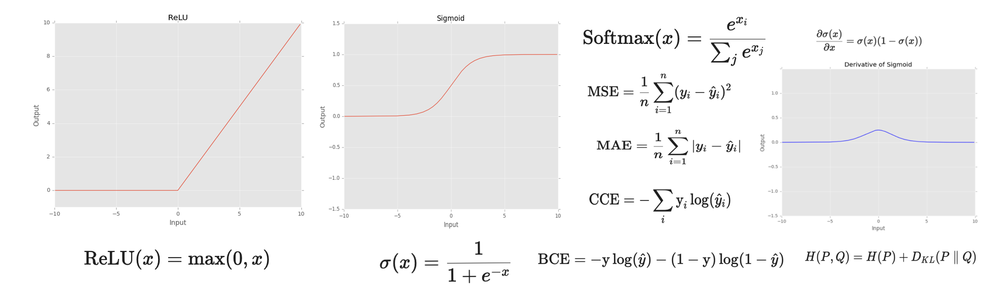
The Rectified Linear Unit activation function or ReLU for short is a piecewise linear function that will output the input directly if it is positive, otherwise, it will output zero.
\[\text{ReLU}(x) = \text{max}(0, x)\]Although ReLU looks like a linear function, it is a nonlinear function allowing complex relationships to be learned and is able to allow learning through all the hidden layers.
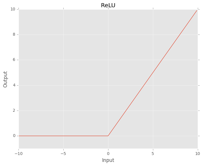
Fig. 1. ReLU function.
There are a lot of variants of the ReLU function, such as Leaky ReLU, Parametric ReLU, and Exponential Linear Unit ( ELU) used for GANs, smoothier loss landscapes and faster model performance respectively.
2. Sigmoid function
The sigmoid function is a smooth, continuous function that maps real-valued inputs to the range \([0, 1]\). That means that the output of the sigmoid function is always between 0 and 1. Large negative numbers will become near to 0, while large positive numbers will become near to 1.
\[ \sigma(x) = \frac{1}{1 + e^{-x}} \]As its range is between 0 and 1, it is ideal for predicting probabilites of an event.
We can understand a classification as a prediction of a probability, but putting a threshold to decide if the prediction is positive or negative.
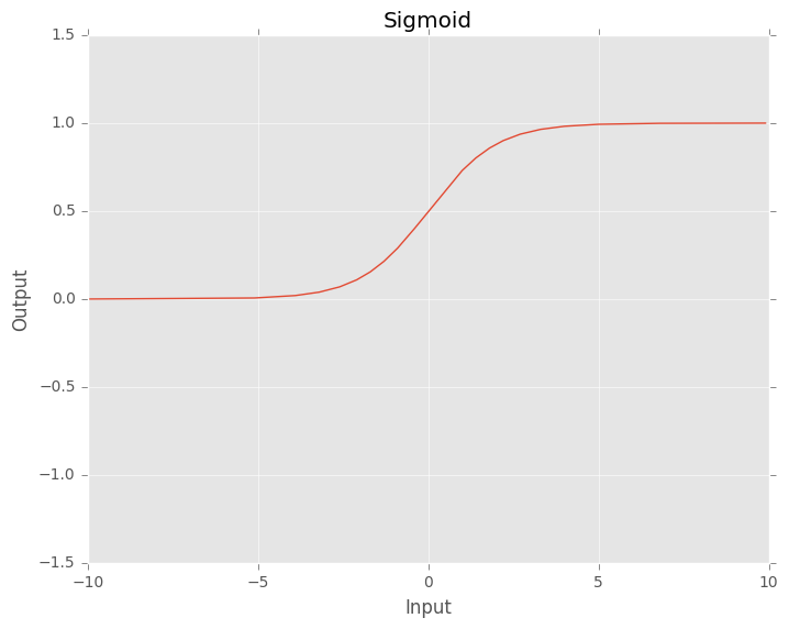
Fig. 2. Sigmoid function.
However, let’s take a look at its derivative:
\[ \frac{\partial \sigma(x)}{\partial x} = \sigma(x) (1 - \sigma(x)) \]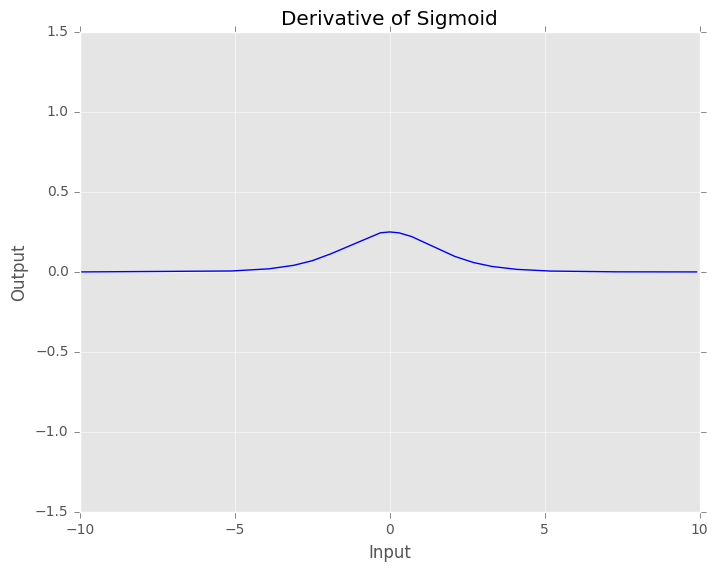
Fig. 3. Derivative of Sigmoid function. We can see the value of the derivative of the sigmoid evaluated at x.
We can see that the gradients of the sigmoid function are really small when \(x \in [-inf, -3] \cup [3, +inf]\). This means that when the input of the neurons are relatively high, the gradients are tiny and the neurons are not able to learn. That is why this activation function is only suitable for final layers.
3. Tanh function
The tanh function is really similar to the sigmoid function, but its output has a range of \([-1, -1]\). Hence, tanh outputs are zero-centered, which leads to better convergence rather than sigmoid.
\[ \tanh(x) = \frac{e^x - e^{-x}}{e^x + e^{-x}} \]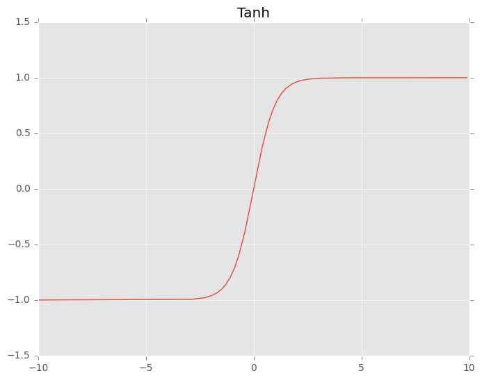
Fig. 3. Derivative of Tanh function.
The derivatives of the tanh are larger than the derivatives of the sigmoid which help us minimize the cost function faster in values near \([-3, 3]\). However, like sigmoid, the gradient values become close to zero for wide range of values. Thus, the network refuses to learn or keeps learning at a very small rate.
\[ \frac{\partial \tanh(x)}{\partial x} = 1 - \tanh^2(x) \]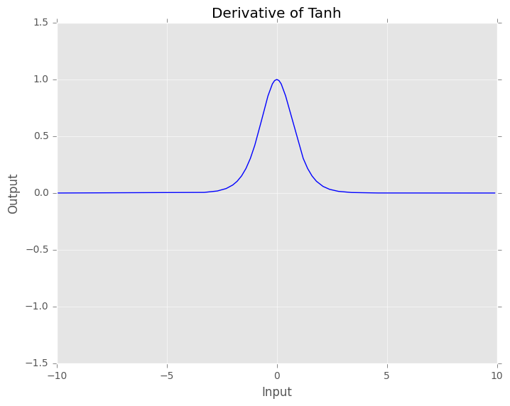
Fig. 3. Derivative of Tanh function. We can see the value of the derivative of the tanh evaluated at x.
The famous problem of having really small gradient values is known as vanishing gradient problem and it has been a problem for a long time.
4. Softmax function
We have seen functions like sigmoid and tanh, that are used to map the output of a neuron to a range of values. However, we can also use a function called softmax to map the output of a layer to a probability distribution.
\[ \text{Softmax}(x) = \frac{e^{x_i}}{\sum_j e^{x_j}} \]Softmax function can be imagined as a combination of multiple sigmoids which can return the probability for a datapoint belonging to each individual class in a multiclass classification problem. The sum of the output of all the probabilities is always 1, since they are normalized. This function is widely used in deep learning to map the output of a layer to a probability distribution and for multi-class one-label classification.
To know which class the neural network thinks the input belongs to, we can use argmax to get the class of the highest probability.
Loss functions
As you may already know, the goal of a neural network is to learn a function that maps data to another data. In order to make the network understand how far or near it is from the desired output, we need to define a loss function. Therefore, loss functions are used to measure the distance between the output of the network and the desired output and the function to optimize.
In this post, we will focus on the most common loss functions used in deep learning, for sure there are many others! In fact, there are many different loss functions for different types of problems. In physics simulations, physic formulas are used to define loss functions.
1. Mean-squared error (MSE) or L2 loss
Mean-squared error (MSE) or L2 loss is a loss function that measures the average squared difference between the predicted values and the actual values. It is commonly used for regression problems where the goal is to predict a continuous value. The formula for MSE is:
\[ \text{MSE} = \frac{1}{n} \sum_{i=1}^{n} (y_i - \hat{y}_i)^2 \]When the expected output of the network is between a range of values, for example, \(y \in [0, 1]\), the MSE loss function can work well with final-activation layers such as sigmoid or tanh. If, for example, the expected output is between \([0, 1000]\), the only needed thing is to multiply the last neuron by 1000. However, when the expected output range is not clear or we have terrible problems with the vanishing gradient problem, we can consider using ReLU instead.
One of the problems of MSE is thet is not robust to outliers in the data and penalizes high and low predictions quadratically.
2. Mean-absolute error (MAE) or L1 loss
Mean-absolute error (MAE) or L1 loss is a loss function that measures the average absolute difference between the predicted values and the actual values.
\[ \text{MAE} = \frac{1}{n} \sum_{i=1}^{n} |y_i - \hat{y}_i| \]It is used when the expected output is a continuous value and we do not want the model to be dominated by outliers. What does that mean? It does not imply that outliers are unimportant; rather, when we use MSE, the error grows quadratically, whereas MAE grows linearly. This means that a single extreme outlier can pull the model much more strongly when using MSE than when using MAE. In contrast, with MAE, outliers have a more limited influence on the training process, allowing the model to focus more on the bulk of the data.
The choice between MAE (Mean Absolute Error) and MSE (Mean Squared Error) is fundamentally about how you want to treat errors and how that impacts optimization.
3. Binary cross-entropy loss
BCE loss is the default loss function used for the binary classification tasks. It is a loss function that measures the probability of the predicted class versus the actual class. For that, it uses the logarithm of the probability of the predicted class. The formula for BCE loss is:
\[ \text{BCE} = -\text{y} \log(\hat{y}) - (1 - \text{y}) \log(1 - \hat{y}) \]where \(y\) is the actual class and \(\hat{y}\) is the predicted class.
BCELoss only requires one output layer (one neuron) to classify the data into two classes. The range of this neuron is between 0 and 1. Hence, the best should use the sigmoid function. As a con, the BCE Loss can only be used for binary classification.
4. Categorical cross-entropy loss
Categorical cross-entropy loss is a loss function that measures the probability of the predicted distribution class versus the actual distribution class. It is used for multi-class classification problems. The formula for Categorical cross-entropy loss is:
\[ \text{CCE} = -\sum_i \text{y}_i \log(\hat{y}_i) \]The main idea here is that we are not only considering one neuron, but the whole resulting output vector of probabilities of the network. Hence, each output neuron of the neural network must be between 0 and 1. But not only that! The sum of the output neurons must be equal to 1. If we have paid attention before, we have seen that the softmax function is used to map the output of a layer to a probability distribution. So, the best way to use this function is to use it as the final-activation layer of the network for this kind of problem.
This loss function is useful when we have multiple classes and we want to measure the probability of each class. For instance, if we want to do a multi-class classification having \(K\) classes but only one accepted class for each sample, we can use a softmax function to map the output of the network to this exact probability distribution.
5. Sparse Categorical cross-entropy loss
Sparse Categorical Cross-Entropy (SCCE) loss is a variant of categorical cross-entropy used for multi-class classification problems where each sample belongs to exactly one class, but the ground-truth labels are provided as integer indices instead of one-hot encoded vectors.
For example, if we have 4 classes, instead of representing the target as:
\[ [0, 0, 1, 0] \]we can simply represent it as:
\[ y = 2 \]where 2 is the index of the correct class.
The loss is defined as:
\[ \text{SCCE} = - \log(\hat{y}_y) \]where \(y\) is the true class index and \(\hat{y}_y\) is the predicted probability assigned to that correct class.
This loss is mathematically equivalent to categorical cross-entropy, but it is more convenient when the labels are already encoded as integers, since we do not need to transform them into one-hot vectors. This can also reduce memory usage when dealing with a large number of classes.
As in categorical cross-entropy, the network output must represent a valid probability distribution. Therefore, the most common final activation function is softmax, which ensures that:
- each output value is between 0 and 1,
- the sum of all output values is equal to 1.
Sparse categorical cross-entropy is commonly used in practice because many datasets already store labels as integers. In frameworks such as PyTorch, this behavior is the default for multi-class classification losses such as
CrossEntropyLoss.
In short, if we have a multi-class classification problem with one valid class per sample:
- use categorical cross-entropy when the labels are one-hot encoded,
- use sparse categorical cross-entropy when the labels are integer class indices.
6. Kullback-Leibler divergence
Kullback-Leibler divergence, also known as KL divergence, is a measure of how different one probability distribution is from another. Instead of comparing a single predicted value against a target value, KL divergence compares two full probability distributions.
It is defined as:
\[ D_{KL}(P \parallel Q) = \sum_i P(i)\log\left(\frac{P(i)}{Q(i)}\right) \]where:
- \(P\) is the true or reference probability distribution,
- \(Q\) is the predicted or approximated probability distribution.
The intuition behind this formula is that it measures how much information is lost when we use \(Q\) to approximate \(P\). If both distributions are identical, the KL divergence is equal to 0. The more different they are, the higher the divergence becomes.
KL divergence is not symmetric, which means that:
\[ > D_{KL}(P \parallel Q) \neq D_{KL}(Q \parallel P) > \]Therefore, changing the order of the distributions changes the result.
KL divergence is strongly related to cross-entropy. In fact, cross-entropy can be decomposed as:
\[ H(P, Q) = H(P) + D_{KL}(P \parallel Q) \]where \(H(P)\) is the entropy of the true distribution. Since \(H(P)\) is constant with respect to the model, minimizing the cross-entropy is equivalent to minimizing the KL divergence between the true and predicted distributions.
This is why cross-entropy is such a natural choice for classification: it encourages the model to make its predicted distribution as close as possible to the target distribution.
KL divergence is especially useful when the target is not just a single correct class, but a full distribution. Some common use cases are:
- Variational Autoencoders (VAEs), where the latent distribution is forced to be close to a prior distribution,
- Knowledge distillation, where a smaller model learns to imitate the soft probability outputs of a larger model,
- Probabilistic modeling, where comparing distributions is more meaningful than comparing scalar values.
In practice, we can think of the difference as follows:
- Cross-entropy losses focus on predicting the correct class,
- KL divergence focuses on matching the full probability distribution.
Therefore, KL divergence is particularly useful when we care not only about the final decision, but also about the structure of the predicted probabilities.