Object detection is one of the most popular tasks in computer vision, since it can be applied to a wide range of applications: robotics, autonomous driving or fault detection. In this post, we will try to give a brief overview of the YOLO algorithm and the components that make it work.
To do that, I have classified the main components of the algorithm into three categories:
- Characteristics based on the model architecture, how YOLO-based models improved the performance by using a new architecture and which are the improvements made.
- Strategies based on the model training, such as the function loss or data augmentation.
- Methods for post-processing the output of the model, such as the non-maximum suppression (NMS) and the confidence threshold.
Two-stage vs One-stage Detectors
Before YOLO, SoTA detectors were based on a two-stage detector: the first stage is used to detect the bounding boxes, and the second stage is used to classify the bounding boxes. This kind of model is called region-based detectors, because they need the region to then run the classification.

Fig. 1. RCNN architecture. (Bhalla, 2022)
In contrast, YOLO is a one-stage detector, YOLO models skip the first stage and runs directly over a dense sampling of possible locations and gives the bounding boxes and the classification all at once. The first idea behind YOLO was to reduce the computational cost of the region-based models (increasing the FPS) although mantaining or decreasing a little bit the performance. This idea was inspired by Single Shot MultiBox Detector (SSD), introduced in 2016.
Frames per second (FPS)
The architecture: Backbone, neck and head
A YOLO model usually has three main parts:
- The backbone network, which extracts features from the input image. The backbone progressively reduces spatial resolution while increasing semantic richness.
- The neck, which combines the feature maps from the backbone with a convolutional layer. So the neck helps the detector handle objects of different sizes.
- The head, which produces the final prediction.

Fig. 2. YOLO-based network architecture. Check image source
These parts are strongly connected to the idea of multi-scale detection. YOLO does not predict bounding boxes from only one feature map. Instead, it preodicts object at different scale resolutions. For example, if the input image has size 640 × 640, a YOLO model may produce three detection scales:
P3 ->  80 x 80  -> small objects
P4 ->  40 x 40  -> medium objects
P5 ->  20 x 20  -> large objects
At the beginning of the backbone, the feature maps have high spatial resolution and contain low-level information, such as edges, corners, textures, and small visual patterns. As the image passes through deeper layers, the spatial resolution decreases, but the semantic meaning of the features increases. The backbone network gives intermediate feature maps to the neck according to the idea of multi-scale detection. Usually the backbone is already pre-trained on a large dataset.
Since the backbone is meant to extract features from the input image in different scales, it is important to create a network that has neither stride operations nor pooling layers, as they can reduce the spatial resolution and semantic information.
The neck takes the feature maps from the backbone and mixes these features so that each detection scale benefits from both.
The detection heads are the final prediction layers. Usually, YOLO has one detection head per scale. Each head predicts bounding boxes (4 values), confidence score (1 value), and class probabilities (C values) for its corresponding feature map. The final prediction output of each head has the shape \(S \times S \times (5B + C) \). If there are 3 different scales, then the output will have three tensors with the previous shape.
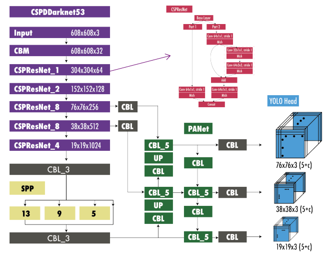
Fig. 3. YOLOv4 Architecture. (Terven & Cordova-Esparza, 2023)
B is the number of bounding boxes per grid cell. It can only be 1, 2 or more. If B is 1, then the model predicts only one bounding box per grid cell.
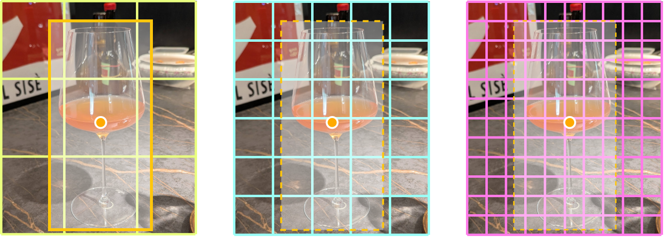
The stride
The stride (S) tells you how much the input of the image has been downsampled. Therefore, each cell in the feature map corresponds to a region of the original image. The \(5B + C\) part of the output is the bounding box (x, y, height and width) and class probabilities.
This is important because YOLO predicts object centers relative to grid cells. Small objects need high-resolution feature maps, so they are usually predicted at lower stride, such as stride 8.

Fig. 4. Example of strides using different scales, with the centroid of the bounding box to determine which is the stride cell of the image to predict.
The confidence score
A YOLO head usually predicts something like: tx, ty, tw, th, objectness, class probabilities
While tx and ty are the predicted center offset of the bounding box and tw and th are the predicted width and
height of the bounding box, the objectness value is the probability that an object exists in this prediction.
The confidence score is commonly calculated by multiplying the objectness value with the class probabilities.
Confidence score is used to remove weak predictions from the output of the model and reduces the number of low-quality detections
The anchor boxes
YOLO models can be divided into two families:
- Anchor-free models, such as (Ge et al., 2021).
- Anchor-based models, such as (Redmon & Farhadi, 2018).
Anchors are predefined box shapes. YOLO models use anchors to predict offsets relative to these boxes. In anchor-based model of three scales, we can have the following anchors:
p3 = [(62, 66), (45, 213), (105, 104)]
p4 = [(196, 76), (153, 143), (96, 316)]
p5 = [(266, 266), (350, 465), (420, 500)]
Anchors are usually defined by classifying the objects of the training set using an unsupervised clustering algorithm, such as k-means.
When using anchors, the output the model is a tensor of shape \(S \times S \times A \times (5B + C) \). Suppose we are
at grid cell (i, j) on a feature map with stride s. The model predicts raw values: tx, ty, tw, th. Hence, a
classical YOLO-style decoding example with anchor (60, 40) is:
bx = (sigmoid(tx) + j) * stride  # e.g. (0.55 + 30) × 8 = 244.4
by = (sigmoid(ty) + i) * stride  # e.g. (0.40 + 20) × 8 = 163.2

bw = anchor_w * exp(tw)  # e.g. 40 × 1.10 = 44.0
bh = anchor_h * exp(th)  # e.g. 60 × 0.82 = 49.2
In modern anchor-free YOLO variants such as YOLOX, anchors may not be used explicitly. Instead, the model directly predicts box distances or center-based boxes.
Decoupled head
YOLOX utilizes a decoupled head, a significant departure from the single-head design in the previous YOLO models.
In traditional YOLO models, the head predicts object classes and bounding box coordinates using the same set of features. This approach simplified the architecture back in 2015, but it had a drawback. It can lead to suboptimal performance, since classification and localization of the object was performed using the same set of extracted features, and thus leads to conflict. Therefore, YOLOX introduced a decoupled head.
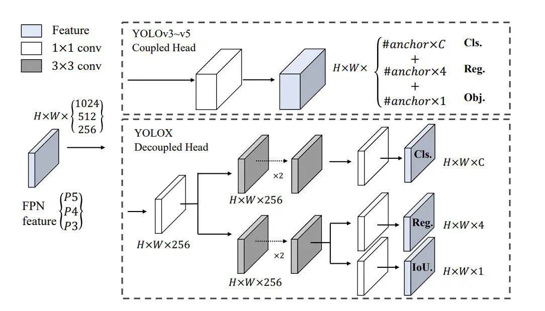
Fig. 5. YOLOX decoupled head architecture. (Ge et al., 2021)
The decoupled head consists of two separate branches:
- Classification Branch. Focuses on predicting the class probabilities for each object in the image.
- Regression Branch. Concentrates on predicting the bounding box coordinates and dimensions for the detected objects.
Model training
Unlike image classification, where the model predicts one label for the whole image, object detection requires solving several problems at the same time: deciding whether an object exists in a given location, estimating the coordinates of its bounding box, and assigning the correct class. For this reason, YOLO training is usually based on a multi-part loss function that combines localization, objectness, and classification terms.
Intersection over Union (IoU)
Intersection over Union (IoU) is a measure of the similarity between two bounding boxes. It is the division between the area of the intersection and the area of the union.
\[IoU = \frac{\text{Area of Intersection}}{\text{Area of union}}\]It is used in several steps of the training process:
- Training loss.
- Anchor assignment.
- Post-processing techniques such as non-maximum suppression (NMS).
- Evaluation metrics such as mAP.

Fig. 6. Intersection over Union (IoU) formula.
mAP — Mean Average Precision
mAP is the standard metric for comparing object detectors across classes and IoU thresholds. For each class, predictions are sorted by confidence score and a precision-recall curve is computed. The area under that curve is the Average Precision (AP) for that class. mAP averages AP over all \(C\) classes:
\[mAP = \frac{1}{C}\sum_{c=1}^{C}AP_c, \qquad AP_c = \sum_{n} (R_n - R_{n-1})\, P_n\]where \(R_n\) is the recall and \(P_n\) the best precision at each confidence threshold.
Loss function
The loss function tells the model how wrong its predictions are during training. The YOLO loss trains the model to solve three tasks at the same time:
- The box loss: localize the object correctly.
- The objectness loss: predict whether an object exists.
- The class loss: classify the object correctly.
A simplified YOLO loss can be written as:
\[ L = \lambda_{\text{box}}L_{\text{box}} + \lambda_{\text{obj}}L_{\text{obj}} + \lambda_{\text{cls}}L_{\text{cls}} \]where \(\lambda_{\text{box}}\), \(\lambda_{\text{obj}}\), and \(\lambda_{\text{cls}}\) are weighting factors used to balance the contribution of each term.
The box loss
The box loss measures how well the predicted bounding box matches the ground-truth box. Older YOLO versions used mean squared error (MSE) over the box coordinates, but modern YOLO models usually use IoU-based losses because they are more directly aligned with the object detection objective. A simple IoU loss can be defined as:
\[ L_{\text{box}} = 1 - IoU(b, \hat{b}) \]where \(b\) is the ground-truth box and \(\hat{b}\) is the predicted box.
However, modern detectors often use more advanced variants such as GIoU, DIoU, or CIoU. For example, CIoU includes not only the overlap between boxes, but also the distance between their centers and their aspect-ratio consistency:
\[ L_{\text{CIoU}} = 1 - IoU + \frac{\rho^2(b, \hat{b})}{c^2} + \alpha v \]where \(\rho^2(b, \hat{b})\) is the squared distance between the centers of the predicted and ground-truth boxes, \(c^2\) is the squared diagonal length of the smallest enclosing box, and \(\alpha v\) penalizes differences in aspect ratio.
The objectness loss
The objectness loss teaches the model whether a prediction contains an object. YOLO makes thousands of predictions per image. Therefore, it is important to balance the false positives. How? By adding weights when the model predicts a positive object. For example, a training implementation may use two different weights:
neg_obj_weight_with_pos: the weight applied to negative predictions in a scale where at least one positive object exists.neg_obj_weight_no_pos: the weight applied to negative predictions in a scale where no positive object exists.
This distinction is useful in multi-scale YOLO training. Suppose that an image contains a small object assigned to the P3 scale, but no objects are assigned to P4 or P5. In that case, P3 contains both positive and negative samples, while P4 and P5 contain only negative samples. If the loss gives too much weight to all negative predictions, the model may learn to predict background everywhere and become too conservative. These weights help balance the objectness loss so that negative examples are useful but do not dominate the training signal.
The class loss
The class loss teaches the model which class is present in a positive prediction. There are two common ways to compute it. If each object belongs to exactly one class, the model can use a softmax activation followed by categorical cross-entropy:
\[ L_{\text{cls}} = - \sum_{c=1}^{C} y_c \log(\hat{p}_c) \]where \(y_c\) is the ground-truth class indicator and \(\hat{p}_c\) is the predicted probability for class \(c\).
However, many YOLO implementations use binary cross-entropy independently for each class:
\[ L_{\text{cls}} = - \sum_{c=1}^{C} \left[ y_c \log(\hat{p}_c) + (1-y_c)\log(1-\hat{p}_c) \right] \]This formulation treats class prediction as \(C\) independent binary classification problems. It is especially useful when multi-label classification is possible, although it is also commonly used in single-label YOLO detectors.
Check that each stride \((S, S)\) has only one positive prediction. Therefore, the model cannot learn to predict two objects in the same location.
Data Augmentation
Data augmentation is another important part of YOLO training. Its goal is to expose the model to more visual variation without manually collecting more data. Common augmentations include random scaling, cropping, horizontal flipping, color jittering, mosaic augmentation, and MixUp.
MixUp combines two images and their labels into a single training example. The resulting image is a weighted combination of both images:
\[ \tilde{x} = \lambda x_1 + (1-\lambda)x_2 \]where \(x_1\) and \(x_2\) are two training images, and \(\lambda\) controls how much each image contributes to the final mixed image.
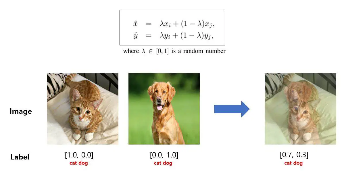
Fig. 5. MixUp Data Augmentation. Check source
MixUp is used for example in YOLOX models and it has been found to be more effective in larger models.
Post-processing
After the model produces its raw predictions, these outputs still need to be converted into final detections. A YOLO model usually predicts many candidate boxes for the same object, many low-confidence boxes, and sometimes overlapping detections from different scales. Post-processing transforms these dense predictions into a clean final set of bounding boxes by applying confidence filtering, decoding the predicted coordinates, and removing duplicated detections with non-maximum suppression.
Non-maximum suppression (NMS)
Non-Maximum Suppression (NMS) is used to remove duplicate detections in bounding box prediction. YOLO often predicts many boxes around the same object. NMS keeps the strongest one and removes highly overlapping boxes.
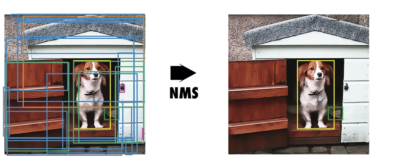
Fig. 6. Non-Maximum Suppression. (Terven & Cordova-Esparza, 2023)
The process is as follows:
- Sort the predictions by their confidence score.
- For each class:
- Keep the box with the highest confidence score.
- Check other boxes with high IoU overlap with the kept box.
- Repeat until all boxes have been processed.
Class-agnostic vs class-aware NMS
Bhalla, D. (2022, June). Region Proposal Network (RPN): A complete guide. ListenData. https://www.listendata.com/2022/06/region-proposal-network.html
Ge, Z., Liu, S., Wang, F., Li, Z., & Sun, J. (2021). YOLOX: Exceeding YOLO series in 2021. arXiv. https://doi.org/10.48550/arXiv.2107.08430
Redmon, J., & Farhadi, A. (2018). YOLOv3: An incremental improvement. arXiv. https://doi.org/10.48550/arXiv.1804.02767
Terven, J., & Cordova-Esparza, D. (2023). A comprehensive review of YOLO architectures in computer vision: From YOLOv1 to YOLOv8 and YOLO-NAS. Machine Learning and Knowledge Extraction, 5, 1680–1716. https://doi.org/10.3390/make5040083
@article{alas2026,
  title   = "Reviewing YOLO: You Only Look Once",
  author  = "Alàs Cercós, Oriol",
  journal = "oriolac.github.io",
  year    = "2026",
  month   = "April",
  url     = "https://oriolac.github.io/posts/20260501-yolo/"
}