In this post we will present an introduction of how Spatial Graph Neural Networks (GNNs) or Graph Convolutional Neural Networks (GCNs) work. First, we are going to define graph data structures. Then, we are going to explain the mechanism on GNNs. And finally, we will explain how to incorporate an attention mechanism in the network.
Notation of GNNs
During the whole text, we will use the notation of GNN as Spatial Graph Neural Network, although GCN or Graph Convolutional Neural Network is another notation to say it. There are other types of GNNs like Spectral Graph Neural Networks, but in this post we will focus on the first mentioned ones.
What are graphs?
Graphs are data structures with two main elements: the nodes and their relationships between elements, named edges. The core of graphs is that we can define very easily the interaction of entities. Here, the links are key to the power of relational-data. Graphs are used in several applications, for instance, in social networks, distribution networks, and state-machines.
First steps
We have already seen three clear concepts:
- Graph. A data type consisting of nodes and edges.
- Nodes/Vertices. Endpoint in a graph, they are also called vertices or points.
- Edges. The link or relationship between nodes.
When trying to describe how is a specific graph, we could always draw the elements and the link between them if necessary. Although it is great to see some properties in a straight-forward way, we could not calculate anything from it. One of the most common mathematical formalisms for describing relations in graphs are adjacency matrices.
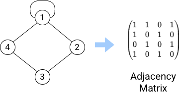
Fig. 1. Adjacency matrix of a graph.
Graphs can be classified as directed or unidrected. In undirected graphs, the adjacency matrix is a symmetric matrix across the diagonals. Each column and row correspond to a node and their values are their corresponding links to the nodes of the graph. For example, in column \(k\) we can see the links of node \(v_k\) and in row \(k\) we can see the same links too, but transposed.
Given two nodes \(v_j\) and \(v_i\), if the value of \(e_{i, j}\) or \(e_{j, i}\) is zero, that means that no link exists between these nodes. Otherwise, there is a link between these nodes.
If the adjacency matrix is not symmetric, we have a directed graph. The links of directed graphs have directions, so that means that a node \(v_j\) can interact to \(v_i\), but it does not have to be the other way around. Directed edges are usually represented by an arrow, denoting a one-way relationship.
\[ G = \begin{pmatrix} 1 & 0 & 0 & 1\\ 0 & 0 & \textcolor{blue}{1} & \textcolor{blue}{1}\\ 0 & \textcolor{red}{0} & 0 & 1\\ 1 & \textcolor{red}{0} & 1 & 0 \end{pmatrix} \qquad \text{This is a directed graph.} \]If not all the non-zero values of the adjacency matrix are one, we are talking about weighted graphs. Weighted graphs can have weighted links.
Other key terms
Other key terms about edges and nodes are:
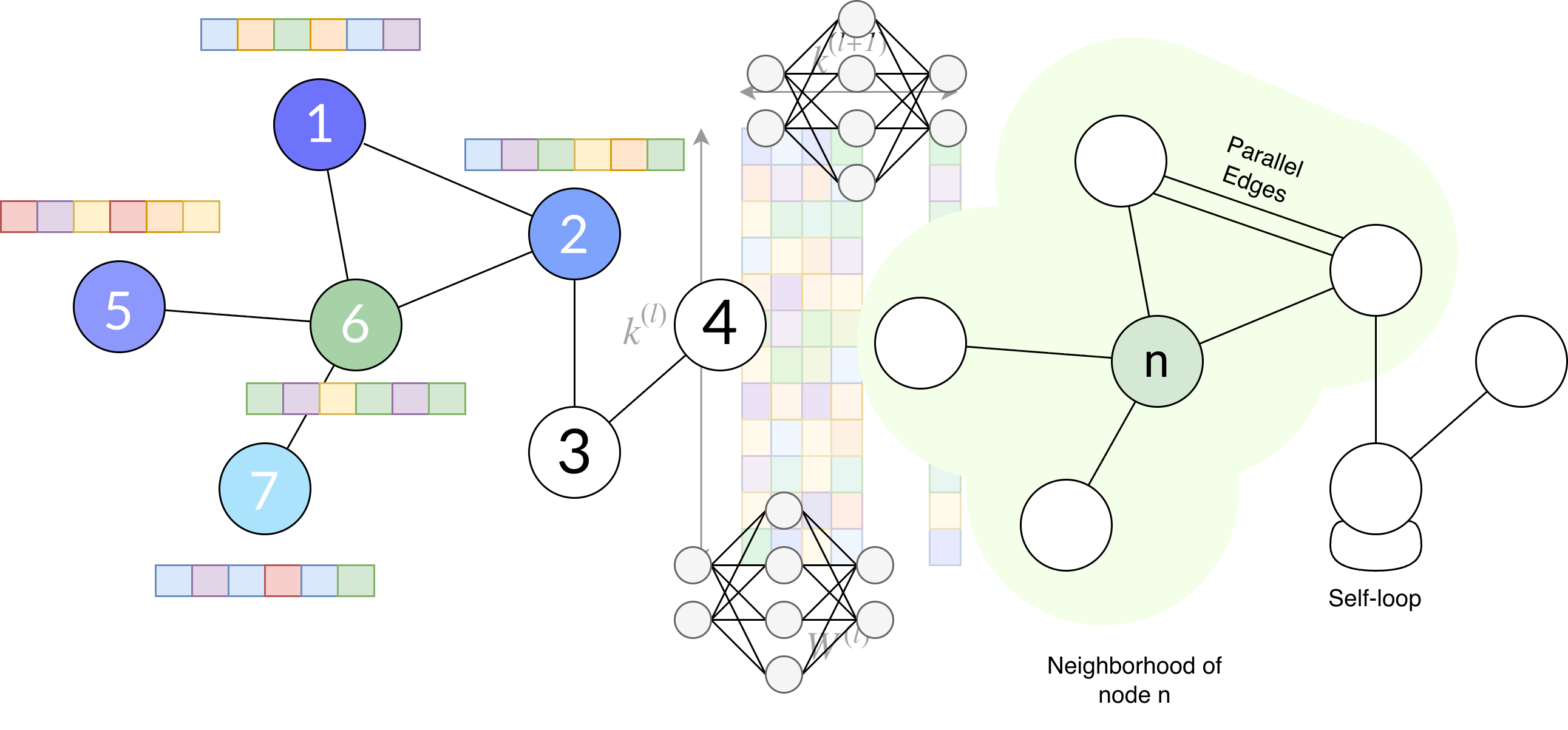
- Self-loop. An edge that connects a node to itself.
- Parallel edges. Multiple edges that connect the same two nodes.
- Joint nodes or neighbours are those nodes that are directly connected via an edge. A node \(v_i\) is adjacent to another node \(v_j\) if there is a edge. The set of all the neighbours from a node is called its neighbourhood.
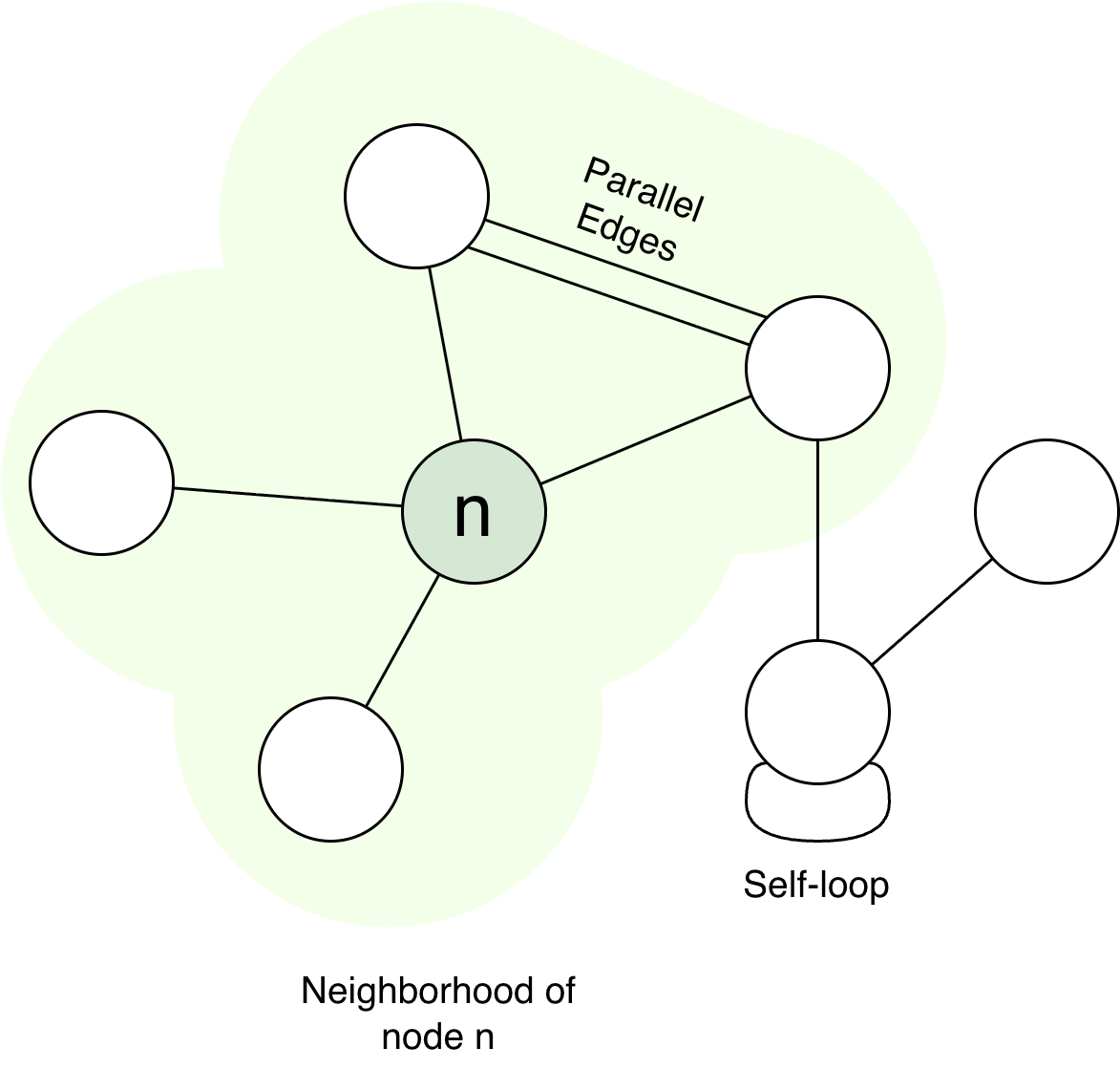
Fig. 2. A graph that has a self-loop, parallel edges. The diagram shows the neighbourhood of node.
Once defined the different kind of graphs depending on the nodes and the edges, we can see other properties checking the structure of a specific node.
- Size is the number of edges.
- Order is the number of nodes.
- The degree of a node is the number of edges associated to a node. It is the count of its adjacent nodes.
- The degree distribution is the distribution of all the degrees of all nodes in a graph. In directed graphs, there are two types of degrees: the in-degrees for edges directed to the node and the out-degrees, for edges directed outward from the node.
- The diameter of a graph is the maximum number of the longest shortest path.
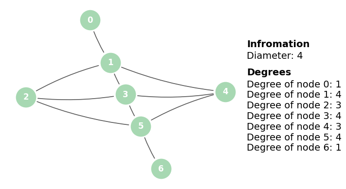
Fig. 3. Degrees and diameter of the graph. The diameter is 4 given the walk (0,1,2,5,6).
- A connected graph is a graph where all its nodes are connected. Otherwise, it is a disconnected graph.
- For a disconnected graph, each disconnected piece is called a component.
- For a directed graph, a strongly connected graph is when it is always possible to reach any node from any
other node. In directed graphs, we can have strongly connected components and weakly connected components.
- Strongly connected components are the subgraphs that are connected to each other and any node in the subgraph can reach any other node in the subgraph.
- Weakly connected components are subgraphs where any node can be reached but not all the nodes can reach each other.
Graph Traversals
When inspecting a graph we might ask ourselves a lot of questions. For example, in a social network how many connections do I have to hop to meet Meryl Streep? In a distribution system, which is the smallest number of hops from one node to another? Which is the largest number of hops without repeating in a graph?
The trip that we have to do to travel from a given node to a second node is called traversal or walk. A walk is open when the ending node is different from the starting node. If we start and end with the same node, we call it closed walk.
A path is a walk when no node is repeated. When the path is closed, we call it cycle. The diameter of a graph is the maximum number of steps of a path. A diameter is also called the longest shortest path.
A trail is when the walk do not repeat edges. A circuit is when we have a closed trail.
How Graph Neural Networks work?
A Graph Neural Network (GNN) is a deep learning model that allows you to represent and learn from graphs (Scarselli et al., 2009). The reason why they were invented is due to the lack of inductive biases in the nature of traditional machine learning and deep learning models such as MLP. In machine learning involving tabular data, images, or text, our data is organized in an expected way, with implicit and more explicit rules. When dealing with tabular data, rows are treated as observations while columns as features. But in graph data, relations between “rows” or instances are meaningful. IN GNNs, we have the information of each node, called embeddings and the links that connects each node to its neighbourhood.
Main idea of GNNs
The essential idea of graph neural networks is to iteratively update the node representations by combining the representations of their neighbours and their own representations.
The main objective of a Graph Neural Network is to encode the data structure to then predict. But, what? There are several tasks that we could come up with, but they can be classified as:
- Node-level tasks. Given a graph, classify the nodes, use regression, or detect anomalies.
- Edge-level tasks. Similar to the node-level tasks, but for edges.
- Graph-level tasks. Graph classification or regression. Graph AutoEncoders (GAE) could be also in this category.
In section 1 we have already understood the importance of the links when defining a graph. GNNs came up to use this nature in the network architecture: use a mechanism to encode and exchange information across the graph structure during the inference: the graph convolutional layers (GCL). The GCN layer \(l\) is mathematically defined as
\[ \mathbf{x}_i^{(l)} = \sum_{j \in \mathcal{N}(i) \cup \{ i \}} \frac{1}{\sqrt{\deg(i)} \cdot \sqrt{\deg(j)}} \cdot \left(\mathbf{W}^{\top} \cdot \mathbf{x}_j^{(l-1)} \right) + \mathbf{b}, \]where neighboring node features are first transformed by a learnable weight matrix \(\mathbf{W}^{\top}\), normalized by their degree, and finally summed up. Lastly, we apply the bias vector to the aggregated output.
However, when we talk unformally about GCL, we talk about a bundle of sequential layers:
- Message Passing layer: where information is aggregated from neighbours and updated for each node.
- Activation Layer: where the information is passed to the next layer.
- Dropout layer: switching off some neurons to improve generalization and performance.
- Normalization Layer: normally Batch Normalization, that means the activated outputs to zero with a variance of 1.
The message-passing method
Message passing is designed specifically for asking about the graph data structure. For each node in the graph, each message passing step represents a communication that spans nodes one hop away. If we want our node representations to take account node from 5 hops from each node, we should need 5 message passing layers.
Message passing can be understood as a form of convolution but applied to the neighbourhood of the nodes instead of a neighbourhood of pixels. Through convolution operators, we are encoding neighbour states to the current node and gathering more global information of the graph.
Inductive biases of GNNs
Hence, Graph Neural Networks can be considered an abstraction of Convolutional Neural Networks.
A popular way to introduce GCLs is to break down the filter into two operations:
- AGGREGATE-NODES. Given a node \(v_i\) and its linked nodes \(\mathcal{N}(v_i)\), we aggregate the information of each neighbour node:
The aggregation function \(AGGREGATE\) is commonly a sum operation, although it can be the mean, minimum, maximum, or multiplication.
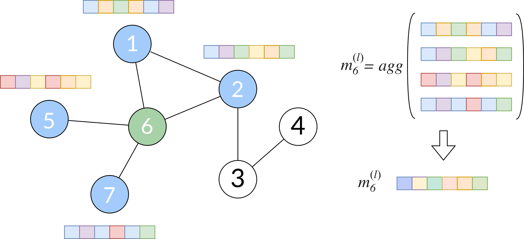
Fig. 4. Aggregate function of node \(6\). This step aggregates the embeddings of the neighbours of the node by multiplying or summing. The resulting value is the message \(m_6^{(l)}\)
- UPDATE-EMBEDDING. Then, we update the embedding of the node \(v_i\) with the aggregated information applying linear transformations:
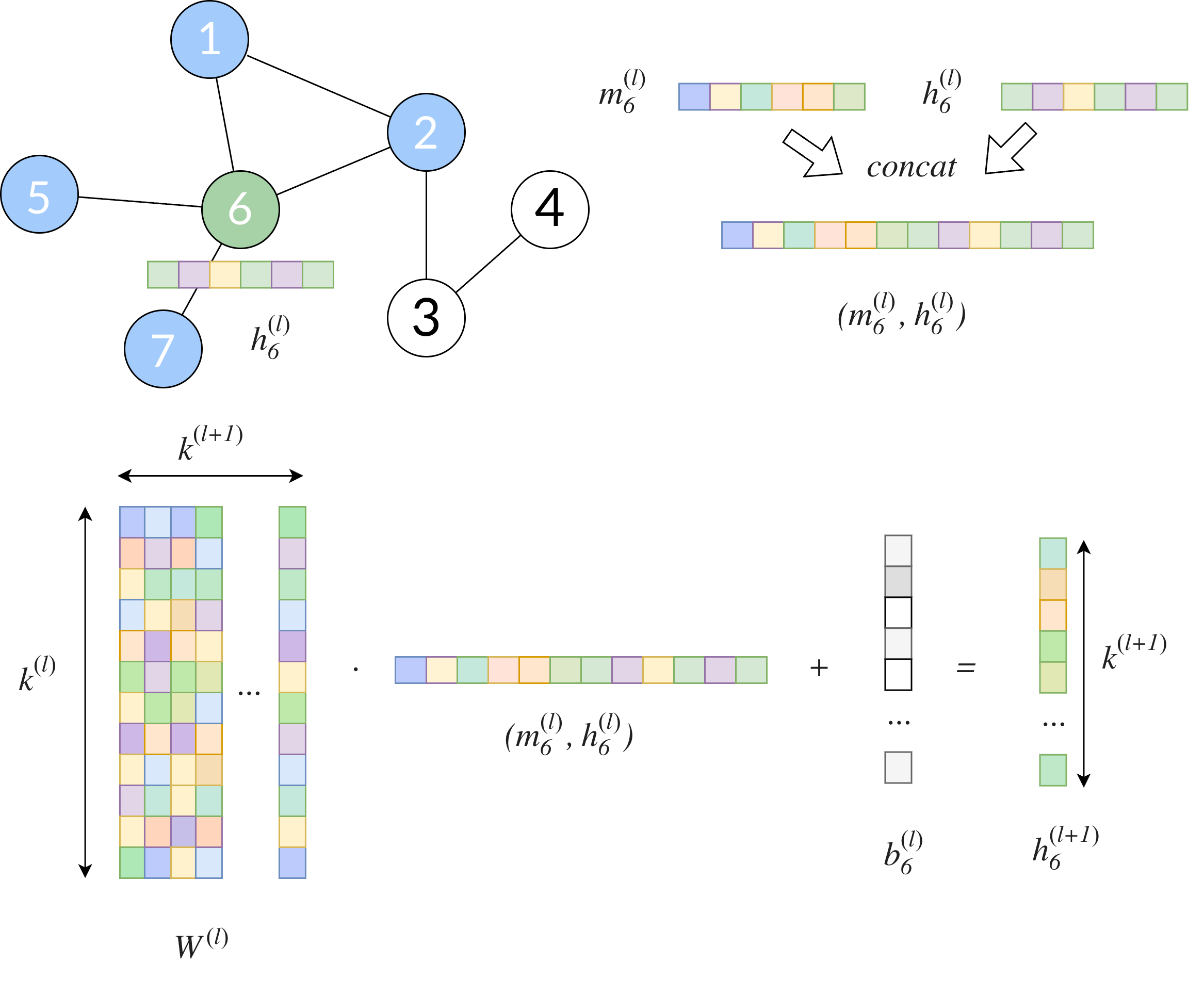
Fig. 5. We concat the current embedding of the node \(6\) with the aggregate message of its neighbours. The resulting value is multiplied by the kernel matrix \(W^{(l)}\) and added to the bias vector \(b^{(l)}\).
Since we will be working on convolutions, a key item must be introduced: the kernel \(W^{(l)}\). The kernel is a matrix that we will be using to transform the input data (from the neighbours) and highlight specific features from them. The kernel is the learnable weight matrix to be optimized by our loss function, along with the bias \(b^{(l)}\).
Inductive biases of GNNs
Graph-based learning techniques focuses on approaches that are permutation invariant or equivariant. This means that the model is not influenced by the ordering of the graph representation. Therefore, if we shuffle the rows and the columns of the adjacency matrix, our results should not change.
Although this example helps to understand how GNNs work at first glance, it is not the most used algorithm. The generic message-passing equation is
\[ \mathbf{x}_i^{(l)} = \gamma^{(l)} \left( \mathbf{x}_i^{(l-1)}, \bigoplus_{j \in \mathcal{N}(i)} \phi^{(l)} \left( \mathbf{x}_i^{(l-1)}, \mathbf{x}_j^{(l-1)}, \mathbf{e}_{j,i} \right) \right) \]where \(\bigoplus\) is the aggregator function, \(\phi^{(l)}\) is the message function at layer \(l\) and \(\gamma^{(l)}\) is the update function. At first, it might look a bit messy since the order is not defined as it is in the example above. So let’s break it by parts again.
- The message function \(\phi^{(l)}\) defines what information each neighbor sends to node \(i\). In the first example, the message function is based solely on sending the embedding information \(h_j^{(l)}\) to node \(i\). Nevertheless, differentiable functions such as MLPs (Multi Layer Perceptrons) can be applied. In addition, the message function can also have as an input the node embedding \(h_i^{(l)}\) as well as the link between the neighbours (useful for weighted graphs). In our example, \[ \phi^{(l)} \left(\mathbf{x}_i^{(l-1)}, \mathbf{x}_j^{(l-1)}, \mathbf{e}_{j,i} \right) = x_j^{(l-1)}\]
- The aggregator function \(\bigoplus\) is the permutation invariant function: sum, max, mean…
- The update function \(\gamma^{(l)}\) is the function that updates the node embedding using the old embedding plus the aggregated message. As you can see, the generic message-passing joins the update with the concat function, which is not needed to be a neither concatenation. Normally, the update functions are also differentiable functions such as MLPs. The following equation is the update function for the first example: \[ \gamma^{(l)} \left(\mathbf{x}_i^{(l-1)}, \bigoplus_{j \in \mathcal{N}(i)} x_j^{(l-1)} \right) = \sigma \left(W^{(l)} \cdot \operatorname{CONCAT} \left(x_i^{(l-1)}, \bigoplus_{j \in \mathcal{N}(i)} x_j^{(l-1)} \right) + b^{(l)} \right)\]
How to apply GNNs to downstreaming tasks?
Since now, we have introduced how to process the data of the nodes with the information of their neighbours. However, we did not apply the information of the nodes to the downstream tasks. In a lot of cases, the GNNs are used only as encoders, while decoders or head networks, such as MLPs, are used to apply the learned graph representation to downstreaming tasks such as node classification, edge prediction, or graph classification.
The GNNs will output the node embeddings, we must think another way around to apply downstream tasks. For example, we can have an MLP to classify the node given the output embeddings given a node (treating then nodes as instances or rows). We could also apply a function to the embeddings of two nodes to get the distance between them and, then, predict if they are connected or not. Regarding graph classification, we could apply global pooling to the embeddings of the nodes to get the final representation of the graph and, then, use an MLP to classify it.
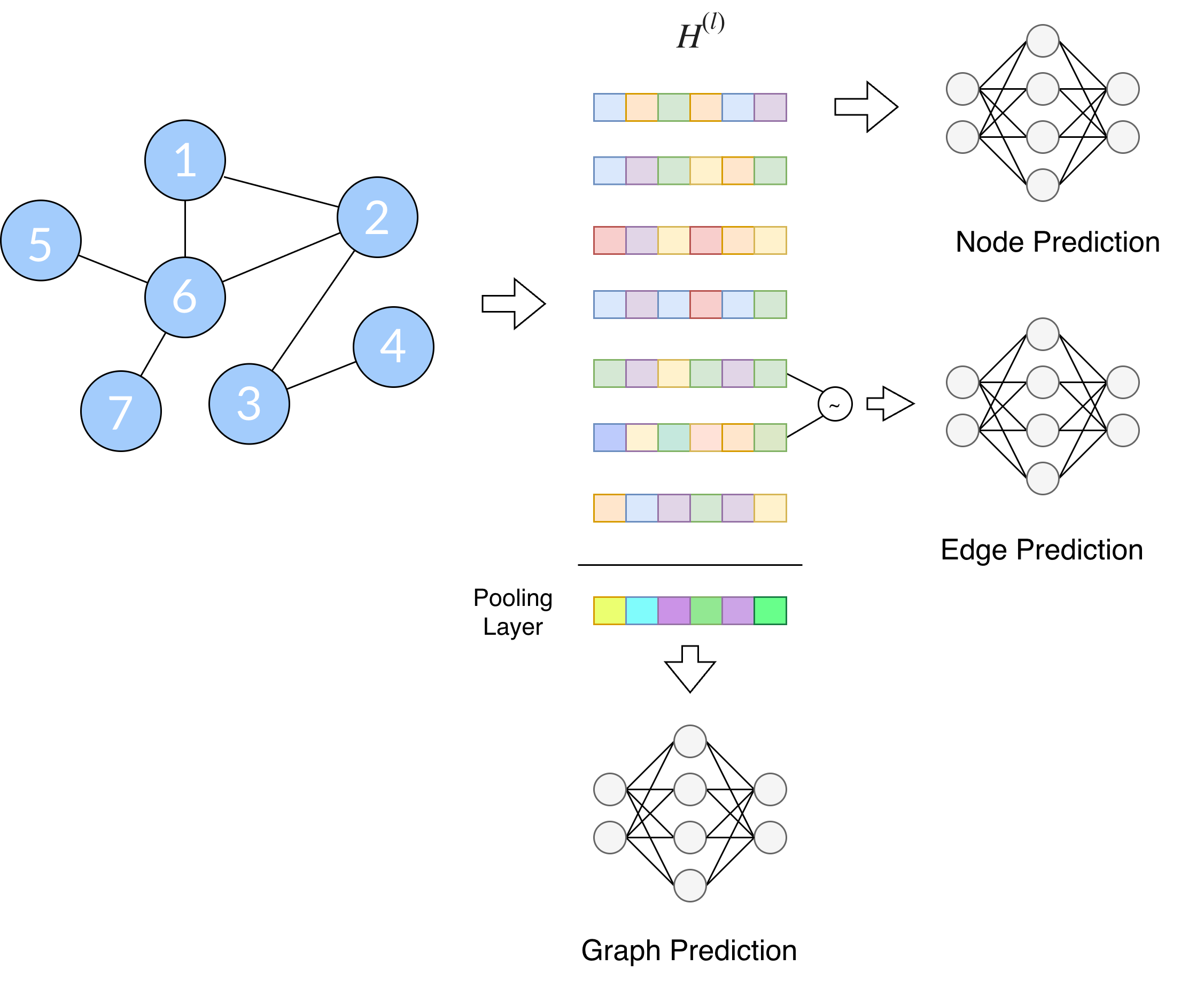
Fig. 6. Given the output of the GNN, we can apply downstream tasks such as node, edge, or graph prediction (regression or classification).
Attention mechanism in GNNs
A GNN with a lot of layers makes the nodes to be more similar to each other, since they will have more global information than first layers. Although it can be great for some tasks, the embedding nodes tend to be more similar to each other, vanishing local information. This problem is called over-smoothing. A way to check if our GNN over-smooths the embeddings of the nodes is to calculate the similarity between each embedding and the average embedding of the nodes. If the similarity of the node and the average is close to 1, it means that the GNN is clearly over-smoothing.
To over-smooth or not to over-smooth?
There are different techniques to avoid over-smoothing such as applying skip connections, similar to U-Net (Ronneberger et al., 2015) or ResNets (He et al., 2016). As you could notice, nodes that have more links tend to be more similar to the average embedding. Specifically, one of the techniques that helps to prevent over-smoothing in these cases is to include attention in the message passing. Therefore, the attention mechanism allows to learn which nodes the network has to put emphasis on.
There are two different attention mechanisms that became popular in the literature: GAT (Veličković et al., 2018) and GATv2 (Brody et al., 2022). The difference between them is where they apply the attention mechanism.
Graph Attention Network (GAT)
Computes the attention weights once per training loop by using individual node and neighborhood features, being static across all layers.
In standard GAT, the unnormalized attention score is usually written as:
\[ e_{i, j} = \text{LeakyReLU} (a^T [W \cdot h_i || W \cdot h_j]) \]where \(a\) is the learnable attention vector, and \(W\) another learnable parameter. We can have also two different learnable parameters \(W_s\) (for the source \(h_i\)) and \(W_t\) (for the target \(h_j\)).
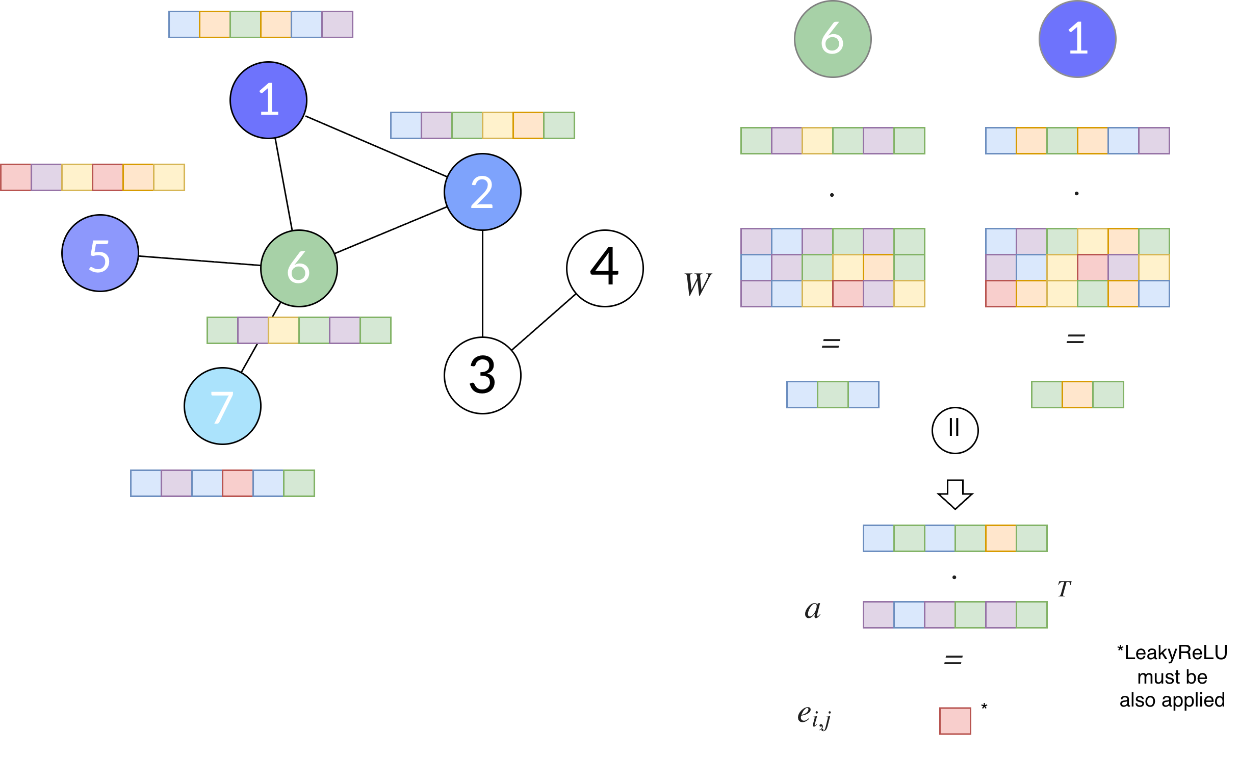
Fig. 7. Unnormalised Attention Score mechanism in GAT.
Then, softmax is applied to normalize the attention scores.
\[ \alpha_{i, j} = \text{softmax}_{j \in \mathcal{N}(i)} (e_{i, j}) \]We can express GAT and GATv2 as specific choices of: \(\phi^{(l)}\). For example:
\[ \phi^{(l)}_{\text{GAT}} (x_i^{(l-1)}, x_j^{(l-1)}, e_{i,j}) = \alpha_{i, j} \cdot x_j^{(l-1)} \]We can also add a learnable parameter to process the attention vector alongside with the neighbour node embedding.
\[ \phi^{(l)}_{\text{GAT}} (x_i^{(l-1)}, x_j^{(l-1)}, e_{i,j}) = \alpha_{i, j} \cdot W^{(l)} \cdot x_j^{(l-1)} \]The problem found in GAT is subtle: the attention vector can be decomposed as:
\[ a^T [W h_i || W h_j] = a_s^T \; W \; h_i + a_t^T \; W \; h_j \]For a fixed source node \(i\), the term \(a_s^T \; W \; h_i \) is constant to all its neighbours \(j\). Therefore, the ranking is mostly determined by \(a_t^T \; W \; h_j \). This kind of attention mechanism is called static, since the ranking of the neighbours does not depend on the source node but only the target node. That means that the attention could be calculated before knowing the link between the nodes. In other words, the attention can be calculated and cached for the whole graph.
GATv2
GATv2 changes the order of operations in the attention mechanism.
\[ e_{i, j} = a^T \text{LeakyReLU} ( W [ h_i || h_j]) = a^T \text{LeakyReLU} ( W_s h_i + W_t h_j) \]As in GAT, we can have two learnable parameters \(W_s\) and \(W_t\) for the attention scores, one for the source node and one for the target node plus the attention vector \(a\). Then, we will apply softmax to normalize the attention scores.
\[ \alpha_{i,j} = \text{softmax}_j \left( e_{i, j} \right) \]The main difference is that the non-linearity is applied before the final attention projection. This allows the source node \(i\) to influence the ranking of the neighbours \(j\). This small change makes GATv2 dynamic attention, showing more expressive attention than GAT while keeping the same parametric cost. Since this mechanism implies calculating the attention for each link, the attention cannot be calculated for the whole graph but for each node. Hence, the number of links from the nodes (the order) increases the cost.
Using the generic message-passing equation, we can rewrite the GATv2 attention function as it was with GAT:
\[ \phi^{(l)}_{\text{GATv2}} (x_i^{(l-1)}, x_j^{(l-1)}, e_{i,j}) = \alpha_{i,j} \; \text{LeakyReLU} ( W_s h_i + W_t h_j), \]but the difference is in the attention score already explained. We can keep \(\gamma^{(l)} \) and \(\bigoplus\) the same.
It is important to note that the attention mechanism adds new learnable parameters to the model, which can be significantly increased in the number of parameters. However, the attention mechanism can help not only to prevent over-smoothing but detect specific important links in the graph.
Conclusion
Graph Neural Networks extend deep learning to data where the relationships between entities are as important as the entities themselves. Instead of processing nodes independently, GNNs exploit the graph structure through message passing, allowing each node to update its representation by combining its own features with information coming from its neighbourhood.
Although GNNs adds a new dimension to deep learning and graph understanding, stacking many message-passing layers can lead to over-smoothing. Attention mechanisms help address this issue by allowing the model to learn which neighbours should contribute more strongly to each node update.
References
Scarselli, F., Gori, M., Tsoi, A. C., Hagenbuchner, M., & Monfardini, G. (2009). The graph neural network model. IEEE Transactions on Neural Networks, 20(1), 61–80. https://doi.org/10.1109/TNN.2008.2005605
He, K., Zhang, X., Ren, S., & Sun, J. (2016). Deep residual learning for image recognition. In Proceedings of the IEEE Conference on Computer Vision and Pattern Recognition (CVPR) (pp. 770–778). IEEE. https://doi.org/10.1109/CVPR.2016.90
Ronneberger, O., Fischer, P., & Brox, T. (2015). U-Net: Convolutional networks for biomedical image segmentation. In N. Navab, J. Hornegger, W. M. Wells, & A. F. Frangi (Eds.), Medical Image Computing and Computer-Assisted Intervention – MICCAI 2015 (pp. 234–241). Springer. https://doi.org/10.1007/978-3-319-24574-4_28
Veličković, P., Cucurull, G., Casanova, A., Romero, A., Liò, P., & Bengio, Y. (2018). Graph attention networks. International Conference on Learning Representations. https://openreview.net/forum?id=rJXMpikCZ
Brody, S., Alon, U., & Yahav, E. (2022). How attentive are graph attention networks? International Conference on Learning Representations. https://openreview.net/forum?id=F72ximsx7C1
Citation
@article{alas2026,
  title   = "Under the Hood of Graph Neural Networks: Message Passing, Over-Smoothing and Attention",
  author  = "Alàs Cercós, Oriol",
  journal = "oriolac.github.io",
  year    = "2026",
  month   = "June",
  url     = "https://oriolac.github.io/posts/20260624-gnns/"
}