During HackUPC 2022, we worked on a time-series forecasting challenge (McKinsey case) to predict sales for multiple product groups. The goal was to support stock planning and cost reduction by generating accurate short-term forecasts from historical sales signals and product information.
Problem
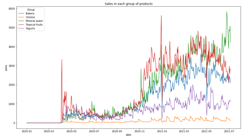
Retail sales exhibit trend shifts, volatility, and category-specific dynamics. In the provided data, several product groups show long periods of low activity followed by abrupt regime changes and sustained growth. This makes purely linear/statistical modeling brittle unless carefully tuned per category.
We framed the task as: predict sales for a target date given product group, price, and previous sales history, and benchmarked classical forecasting against deep sequence modeling.
Constraints
- Hackathon timebox: we needed a working, validated pipeline quickly.
- Heterogeneous categories: each product group behaves differently (scale, spikes, growth rate).
- Windowing decisions: defining lookback length and supervision setup was a key difficulty (sequence-to-one forecasting).
Approach
Pipeline / Architecture
Data understanding & EDA
- Visualized sales trajectories per product group to detect scale differences and regime changes.
Preprocessing
- Aggregation by product group. We simplified the problem since a lot of detailed patterns were underneath the data.
- Train/test split consistent with time-series forecasting (no random shuffling)
- Normalization to stabilize training across categories

Sales in each group of products.
Modeling
- ARIMA per group (baseline)
- RNN/LSTM with configurable lookback window (deep model)
Evaluation
- Metric: MSE
- Qualitative inspection via predicted-vs-real plots per category.
Export
- Generated predictions and saved outputs for submission (e.g.,
response.csvin the reference implementation).
- Generated predictions and saved outputs for submission (e.g.,
Modelling
We implemented two complementary forecasting tracks:
1) ARIMA
We used ARIMA as a fast, interpretable baseline to establish “minimum viable” performance and to expose failure modes ( e.g., sensitivity to abrupt changes). In our internal evaluation, the ARIMA approach achieved MSE ≈ 109.3 on the test setting we reported. ARIMA provided a simple baseline but behaved like a “recent-pattern replicator”, struggling to generalize when the underlying dynamics shifted.

Arima forecasting in test.
2) RNN/LSTM forecaster
We trained an RNN/LSTM-based model using sliding windows over historical sales (and available signals such as price/category), optimized for MSE. This model handled non-linear dynamics and regime shifts better in our experiments, reaching MSE ≈ 0.02 in the reported test evaluation.

RNN forecasting in test.
Results
- The ARIMA baseline struggled to fully track abrupt changes and complex dynamics in some categories (reported MSE 109.3).
- The RNN/LSTM produced substantially tighter fits in our reported evaluation (reported MSE 0.02) and visually tracked the series more closely across time.
What I’d improve next
- Walk-forward validation (rolling-origin evaluation) to reduce the risk of optimistic splits.
- A single model that learns across all groups. Instead of training separate small models (or heavily category-tuned configurations), train a unique global RNN that learns shared temporal patterns across categories and uses category embeddings (and other metadata) to specialize per group.
- Probabilistic forecasts (prediction intervals) for stock decisions, not just point estimates.
- Exogenous drivers (promotions, holidays, weather, store signals) if available.
- Hierarchical forecasting: enforce coherence between product-level and group-level totals.
- Modern sequence models (Temporal CNNs or Transformers) as an upgrade path beyond RNNs. Try architectures that are typically stronger and easier to scale for forecasting or Modern forecasting libraries/models designed for heterogeneous series.